Page 780 - The Mechatronics Handbook

0066_Frame_C24 Page 28 Thursday, January 10, 2002 3:45 PM

i (t) R 1 Op.Amp.
R1
v (t)
+
+ v (t) R 3
−
−
−
v (t) C 1 2 R C 3
i v (t)
v (t) o
C3

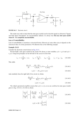
FIGURE 24.13 Electronic circuit.

The reader may wish to check that the state space models used to describe signals in subsection “Signals
and State Space Description” are uncontrollable. Indeed, it is always true that any state space model
where B = 0 is completely uncontrollable.
Loss of Controllability
Lack of controllability is sometimes a structural feature. However, in some other cases, it depends on the
numerical value of certain parameters. We illustrate this in the following example.

Example 24.13
Consider the electronic circuit shown in Fig. 24.13.
We first build a state space model for the circuit. We choose, as state variables, x 1 (t) = i R1 (t) and x 2 (t) =
v C3 (t). Using first principles on the left half of the circuit we have that

d
v +
i C1 = C 1 ----- v i –( v + ), i R1 = v i – v + i R2 = -----, i C1 = i R2 – i R1 (24.160)
--------------,
dt R 1 R 2
This yields
di R1 t() ( R 1 + R 2 ) 1
---------------- = −----------------------i R1 t() + -----------------v i t() (24.161)
dt C 1 R 1 R 2 C 1 R 1 R 2
v + t() = −R 1 i R1 t() + v i t() (24.162)

And, similarly, from the right half of the circuit we obtain
dv C3 t() 1 1
----------------- = −-----------v C3 t() + -----------v − t() (24.163)
dt R 3 C 3 R 3 C 3

v o t() = v C3 t() (24.164)
The (ideal) operational amplifier ensures that v + (t) = v − (t), so we can combine the state space models
given in Eqs. (24.161)–(24.164) to obtain

di () ( R + R ) 1
t
2
1
R1
----------------- – ----------------------- 0 i R1 t() ------------------
dt = C R R 2 + C R R 2 v i t() (24.165)
1
1
1
1
dv () R 1 v C3 t() 1
t
1
C3
------------------ – ------------ – ------------ ------------
dt R C 3 R C 3 C R 3
3
3
3
v o t() = [ 01] i R1 t() (24.166)
v C3 t()
©2002 CRC Press LLC