Page 782 - The Mechatronics Handbook

0066_Frame_C24 Page 30 Thursday, January 10, 2002 3:45 PM

It is important to emphasize that the existence of the integral defined in (24.172) is guaranteed only
if the eigenvalues of A have negative real part, i.e., the system must be stable.
Also, the controllability gramian P defined in (24.172) satisfies the Lyapunov equation

T
T
AP + PA + BB = 0 (24.173)
For discrete-time systems we have the following equations for the controllability gramian:

∞
P d ∑ A d B d B d A d ) (24.174)
=
(
T k
T
k
k=0
which satisfies
T T
A d P d A d – P d + B d B d = 0 (24.175)

The sum defined in (24.174) is bounded if and only if the discrete-time system is stable, i.e., its
eigenvalues lie inside the unit disc.

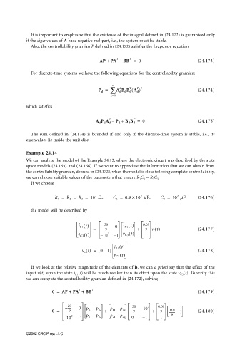
Example 24.14
We can analyze the model of the Example 24.13, where the electronic circuit was described by the state
space models (24.165) and (24.166). If we want to appreciate the information that we can obtain from
the controllability gramian, defined in (24.172), when the model is close to losing complete controllability,
we can choose suitable values of the parameters that ensure R 1 C 1 ≈ R 3 C 3 .
If we choose

3
3
R 1 = R 2 = R 3 = 10 Ω, C 1 = 0.9 × 10 mF, C 3 = 10 mF (24.176)
3
the model will be described by

i R1 t() – 20 0 i R1 t() 0.01
˙
-----
----------
= 9 + 9 v i t() (24.177)
v ˙ C3 t() – 10 3 – 1 v C3 t() 1
i R1 t()
v o t() = [ 01] (24.178)
v C3 t()

If we look at the relative magnitude of the elements of B, we can a priori say that the effect of the
input u(t) upon the state i R1 (t) will be much weaker than its effect upon the state v C3 (t). To verify this
we can compute the controllability gramian defined in (24.172), solving

T
0 = AP + PA + BB T (24.179)

20 20 3 0.01
– ----- 0 p 11 p 12 – ----- – 10 ----------
0 = 9 p 11 p 12 + 9 + 9 0.01 (24.180)
---------- 1
3 p 21 p 22 p 21 p 22 9
– 10 – 1 0 – 1 1

©2002 CRC Press LLC