Page 786 - The Mechatronics Handbook

0066_Frame_C24 Page 34 Thursday, January 10, 2002 3:45 PM

Example 24.16
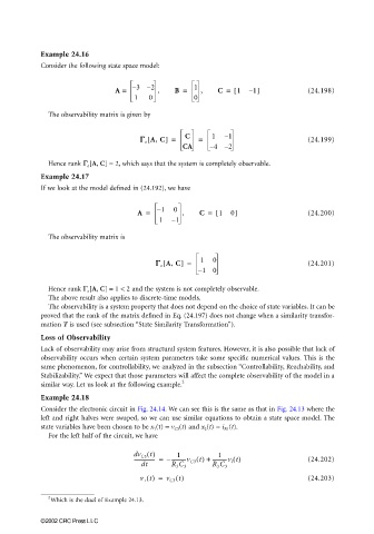
Consider the following state space model:

A = – 3 – 2 , B = 1 , C = 1 [ – 1] (24.198)
1 0 0

The observability matrix is given by

[
ΓΓ Γ Γ A, C] = C = 1 – 1 (24.199)
o
CA – 4 – 2
Hence rank ΓΓ ΓΓ [A, C] = 2, which says that the system is completely observable.
o
Example 24.17
If we look at the model defined in (24.192), we have

– 1 0
A = , C = 1 [ 0] (24.200)
1 – 1

The observability matrix is

ΓΓ Γ Γ A, C] = 1 0 (24.201)
[
o
– 1 0
Hence rank ΓΓ ΓΓ [A, C] = 1 < 2 and the system is not completely observable.
o
The above result also applies to discrete-time models.
The observability is a system property that does not depend on the choice of state variables. It can be
proved that the rank of the matrix defined in Eq. (24.197) does not change when a similarity transfor-
mation T is used (see subsection “State Similarity Transformation”).

Loss of Observability
Lack of observability may arise from structural system features. However, it is also possible that lack of
observability occurs when certain system parameters take some specific numerical values. This is the
same phenomenon, for controllability, we analyzed in the subsection “Controllability, Reachability, and
Stabilizability.” We expect that those parameters will affect the complete observability of the model in a
2
similar way. Let us look at the following example.
Example 24.18
Consider the electronic circuit in Fig. 24.14. We can see this is the same as that in Fig. 24.13 where the
left and right halves were swaped, so we can use similar equations to obtain a state space model. The
state variables have been chosen to be x 1 (t) = v C3 (t) and x 2 (t) = i R1 (t).
For the left half of the circuit, we have

dv C3 t() 1 1
----------------- = −-----------v C3 t() + -----------v i t() (24.202)
dt R 3 C 3 R 3 C 3
v + t() = v C3 t() (24.203)

2
Which is the dual of Example 24.13.

©2002 CRC Press LLC