Page 790 - The Mechatronics Handbook

0066_Frame_C24 Page 38 Friday, January 18, 2002 5:38 PM

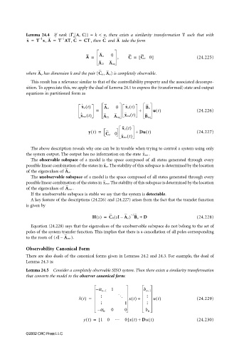
Lemma 24.4 If rank {ΓΓ ΓΓ [A, C]} = k < n, there exists a similarity transformation T such that with
o
1
–
1
–
x = T x, A = T AT, C = CT , then C and A take the form
A = A o 0 , C = [ C o 0] (24.225)
A 21 A no
has dimension k and the pair (C o, A o) is completely observable.
where A o
This result has a relevance similar to that of the controllability property and the associated decompo-
sition. To appreciate this, we apply the dual of Lemma 24.1 to express the (transformed) state and output
equations in partitioned form as

x o t() A o 0 x o t() B o
˙
= + u t() (24.226)
˙ x no t() A 21 A no x no t() B no
x o t()
y t() = + Du t() (24.227)
C o 0
x no t()

The above description reveals why one can be in trouble when trying to control a system using only
.
the system output. The output has no information on the state x no
The observable subspace of a model is the space composed of all states generated through every
possible linear combination of the states in . The stability of this subspace is determined by the location
x o
.
of the eigenvalues of A o
The unobservable subspace of a model is the space composed of all states generated through every
. The stability of this subspace is determined by the location
possible linear combination of the states in x no
.
of the eigenvalues of A no
If the unobservable subspace is stable we say that the system is detectable.
A key feature of the descriptions (24.226) and (24.227) arises from the fact that the transfer function
is given by
1
–
H s() = C 0 sIA o) B o + D (24.228)
(
–
Equation (24.228) says that the eigenvalues of the unobservable subspace do not belong to the set of
poles of the system transfer function. This implies that there is a cancellation of all poles corresponding
–
to the roots of (sIA no ).
Observability Canonical Form
There are also duals of the canonical forms given in Lemmas 24.2 and 24.3. For example, the dual of
Lemma 24.3 is:
Lemma 24.5 Consider a completely observable SISO system. Then there exists a similarity transformation
that converts the model to the observer canonical form:

– α n−1 1 b n−1
x ˙ t() = O xt() + ut() (24.229)
1
– α 0 0 0 b 0

yt() = [ 10 … 0]xt() + Dut() (24.230)

©2002 CRC Press LLC