Page 793 - The Mechatronics Handbook

0066_Frame_C24 Page 41 Thursday, January 10, 2002 3:46 PM

u(t) y(t)
System
^ +
+ x (t)
B (sI-A) -1 C
+ -
J

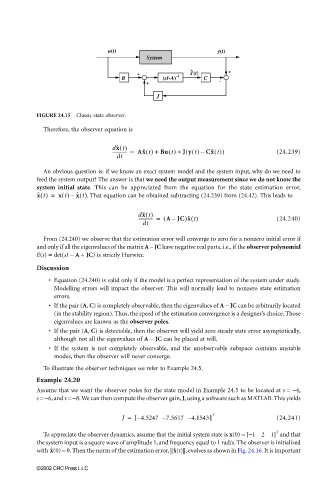
FIGURE 24.15 Classic state observer.
Therefore, the observer equation is

dx ˆ t() Ax ˆ t() + Bu t() + Jy t() Cx ˆ t()) (24.239)
------------- =
(
dt –
An obvious question is: if we know an exact system model and the system input, why do we need to
feed the system output? The answer is that we need the output measurement since we do not know the
system initial state. This can be appreciated from the equation for the state estimation error,
–
x ˜ t() = x t() x ˆ t() . That equation can be obtained subtracting (24.239) from (24.42). This leads to

dx ˜ t()
------------- = ( AJC)x ˜ t() (24.240)
–
dt
From (24.240) we observe that the estimation error will converge to zero for a nonzero initial error if
and only if all the eigenvalues of the matrix A − JC have negative real parts, i.e., if the observer polynomial
E(s) = det(sI − A + JC) is strictly Hurwitz.
Discussion
• Equation (24.240) is valid only if the model is a perfect representation of the system under study.
Modelling errors will impact the observer. This will normally lead to nonzero state estimation
errors.
• If the pair (A, C) is completely observable, then the eigenvalues of A − JC can be arbitrarily located
(in the stability region). Thus, the speed of the estimation convergence is a designer’s choice. Those
eigenvalues are known as the observer poles.
• If the pair (A, C) is detectable, then the observer will yield zero steady state error asymptotically,
although not all the eigenvalues of A − JC can be placed at will.
• If the system is not completely observable, and the unobservable subspace contains unstable
modes, then the observer will never converge.
To illustrate the observer techniques we refer to Example 24.5.
Example 24.20
Assume that we want the observer poles for the state model in Example 24.5 to be located at s = −4,
s = −6, and s = −8. We can then compute the observer gain, J, using a software such as MATLAB. This yields

J = – [ 4.5247 – 7.5617 – 4.1543] T (24.241)

T
To appreciate the observer dynamics, assume that the initial system state is x(0) = [−121] and that
the system input is a square wave of amplitude 1, and frequency equal to 1 rad/s. The observer is initialized
with (0) = 0. Then the norm of the estimation error, || (t)||, evolves as shown in Fig. 24.16. It is importantx ˆ x ˆ

©2002 CRC Press LLC