Page 798 - The Mechatronics Handbook

0066_Frame_C24 Page 46 Thursday, January 10, 2002 3:46 PM

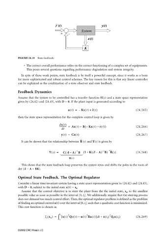
r (t) y(t)
System
+ -
x(t)

K

FIGURE 24.19 State feedback.

• The correct overall performance relies on the correct functioning of a complex set of equipments.
This poses several questions regarding performance degradation and system integrity.

In spite of these weak points, state feedback is by itself a powerful concept, since it works as a basis
for more sophisticated and robust control schemes. The key reason for this is that any linear controller
can be explained as the combination of a state observer and state feedback.

Feedback Dynamics
Assume that the system to be controlled has a transfer function H(s) and a state space representation
given by (24.42) and (24.43), with D = 0. If the plant input is generated according to
u t() = – Kx t() + r t() (24.265)

then the state space representation for the complete control loop is given by

dx t()
------------- = Ax t() + B – Kx t() + r t()) (24.266)
(
dt
y t() = Cx t() (24.267)

It can be shown that the relationship between R (s) and Y(s) is given by

Y s() = C sIA) B ( I + K sIA) B) R s() (24.268)
–
(
1
1
(
–
1
–
–
–
      
H s()
This shows that the state feedback loop preserves the system zeros and shifts the poles to the roots of
det (sI − A + BK).
Optimal State Feedback. The Optimal Regulator
Consider a linear time invariant system having a state space representation given by (24.42) and (24.43),
with D = 0, subject to the initial state x(0) = x o .
Assume that the control objective is to steer the plant from the the initial state, x o , to the smallest
possible value as soon as possible in the interval [0, t f ]. We additionally require that the steering process
does not demand too much control effort. Then, the optimal regulator problem is defined as the problem
of finding an optimal control u(t) over the interval [0, t f ] such that a quadratic cost function is minimized.
This cost function is chosen as
T
J u x o = ∫ t f [ x t() Qxt() + u t() Ru t()] t + x t f () Q f x t f () (24.269)
()
T
T
d
0
©2002 CRC Press LLC