Page 799 - The Mechatronics Handbook

0066_Frame_C24 Page 47 Thursday, January 10, 2002 3:46 PM

where Q ∈ n×n , Q f ∈ n×n are symmetric nonnegative definite matrices and R ∈ m×m is a symmetric
positive definite matrix. The requirements on the weighting matrices are set so that the cost function
makes sense. For instance, if Q is allowed to be negative, then the optimal cost could even be negative
while the state could grow unbounded in magnitude. Also, if we allow R to have eigenvalues at the origin
(i.e., R is allowed to be a nonnegative definite matrix, instead of requiring it to be a strictly positive definite
matrix) then the control u(t) could also grow unbounded (in the directions of the associated eigenvectors)
without that situation being revealed by the cost function.
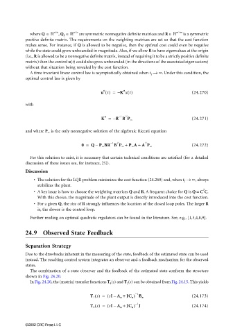
A time invariant linear control law is asymptotically obtained when t f → ∞ . Under this condition, the
optimal control law is given by

u t() = – K xt() (24.270)
o
o
with

K = – R B P ∞ (24.271)
−1
T
o
and where P ∞ is the only nonnegative solution of the algebraic Riccati equation

0 = Q P ∞ BR B P ∞ + P ∞ A + A P ∞ (24.272)
−1
T
T
–
For this solution to exist, it is necessary that certain technical conditions are satisfied (for a detailed
discussion of these issues see, for instance, [5]).
Discussion
• The solution for the LQR problem minimizes the cost function (24.269) and, when t f → ∞ , always
stabilizes the plant.
T
• A key issue is how to choose the weighting matrices Q and R. A frequent choice for Q is Q = C C.
With this choice, the magnitude of the plant output is directly introduced into the cost function.
• For a given Q, the size of R strongly influences the location of the closed loop poles. The larger R
is, the slower is the control loop.

Further reading on optimal quadratic regulators can be found in the literature. See, e.g., [1,3,4,8,9].

24.9 Observed State Feedback

Separation Strategy
Due to the drawbacks inherent in the measuring of the state, feedback of the estimated state can be used
instead. The resulting control system integrates an observer and a feedback mechanism for the observed
states.
The combination of a state observer and the feedback of the estimated state conform the structure
shown in Fig. 24.20.
In Fig. 24.20, the (matrix) transfer functions T 1 (s) and T 2 (s) can be obtained from Fig. 24.15. This yields

T 1 s() = ( sIA o + JC o ) B o (24.173)
−1
–
−1
T 2 s() = ( sIA o + JC o ) J (24.174)
–

©2002 CRC Press LLC