Page 802 - The Mechatronics Handbook

0066_Frame_C25 Page 1 Wednesday, January 9, 2002 7:05 PM

25

Response of Dynamic

Systems

25.1 System and Signal Analysis
Continuous Time Systems • Discrete Time Systems
• Laplace and z-Transform • Transfer Function Models
25.2 Dynamic Response
Pulse and Step Response • Sinusoid and
Frequency Response
25.3 Performance Indicators for Dynamic Systems
Raymond de Callafon Step Response Parameters • Frequency Domain
University of California Parameters

25.1 System and Signal Analysis

In dynamic system design and analysis it is important to predict and understand the dynamic behavior
of the system. Examining the dynamic behavior can be done by using a mathematical model that describes
the relevant dynamic behavior of the system in which we are interested. Typically, a model is formulated
to describe either continuous or discrete time behavior of a system. The corresponding equations that
govern the model are used to predict and understand the dynamic behavior of the system.
A rigorous analysis can be done for relatively simple models of a dynamic system by actually computing
solutions to the equations of the model. Usually, this analysis is limited to linear first and second order
models. Although limited to small order models, the solutions tend to give insight in the typical responses
of a dynamic system. For more complicated, higher order and possibly nonlinear models, numerical
simulation tools provide an alternative for the dynamic system analysis.
In the following we review the analysis of linear models of discrete and continuous time dynamic
systems. The equations that describe and relate continuous and discrete time behavior are presented. For
the analysis of continuous time systems extensive use is made of the Laplace transform that converts
linear differential equations into algebraic expressions. For similar purposes, a z-transform is used for
discrete time systems.

Continuous Time Systems

Models that describe the linear continuous time dynamical behavior of a system are usually given in the
form of differential equations that relate an input signal u(t) to an output signal y(t). The differential
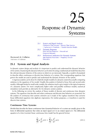
equation of a time invariant linear continuous time model has the general format

n a j n b k
∑ a j ------ yt() = ∑ b j ------ ut() (25.1)
d
d
dt j dt j
j=0 j=0

©2002 CRC Press LLC