Page 800 - The Mechatronics Handbook

0066_Frame_C24 Page 48 Thursday, January 10, 2002 3:46 PM

r (t) u(t) y(t)
System
+ -

T T
1 2
+ +

^
x(t)
K

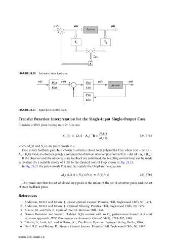
FIGURE 24.20 Estimated state feedback.

r(t) r (t) u(t) y(t)
P(s) + E(s)
System
E(s) L(s)
-
P(s)
E(s)

FIGURE 24.21 Equivalent control loop.

Transfer Function Interpretation for the Single-Input Single-Output Case
Consider a SISO plant having transfer function

N o s()
(
G o s() = C sIA o ) B = -------------- (24.275)
−1
–
M o s()
where M o (s) and N o (s) are polynomials in s.
First, a state feedback gain, K, is chosen to obtain a closed loop polynomial F(s), where F(s) = det (sI −
A o + B o K). Next, an observer gain, J, is computed to obtain an observer polynomial E(s) = det (sI − A o + JC o ).
If the observer and the observed state feedback are combined, the resulting control loop can be made
r
equivalent (by a suitable choice of (t)) to the classical control loop shown in Fig. 24.21.
In Fig. 24.21 the polynomials P(s) and L(s) satisfy the Diophantine equation
M o s()Ls() + N o s()Ps() = Es()Fs() (24.276)

This result says that the set of closed loop poles is the union of the set of observer poles and the set
of state feedback poles.

References

1. Anderson, B.D.O. and Moore, J., Linear optimal Control. Prentice-Hall, Englewood Cliffs, NJ, 1971.
2. Anderson, B.D.O. and Moore, J., Optimal Filtering. Prentice-Hall, Englewood Cliffs, NJ, 1979.
3. Athans, M. and Falb, P., Optimal Control. McGraw HIll, 1966.
4. Dennis Bernstein and Wassim Haddad. LQG control with an H ∞ performance bound: A Riccati
equation approach. IEEE Transactions on Automatic Control, 34(3): L293–305, 1989.
5. Bittanti, S., Laub, A.J., and Willems, J.C., The Riccati Equation. Springer Verlag, Berlin, 1996.
6. Dorf, R.C. and Bishop, R., Modern Control Systems. Prentice-Hall, Englewood Cliffs, NJ, 1997.

©2002 CRC Press LLC