Page 795 - The Mechatronics Handbook

0066_Frame_C24 Page 43 Thursday, January 10, 2002 3:46 PM

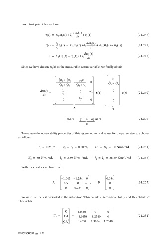
From first principles we have

dw 1 t()
t t() = D 1 w 1 t() + I 1 ---------------- + t 1 t() (24.246)
dt
dw 2 t()
t t() = ----t 1 t() = D 2 w 2 t() + I 2 ---------------- + K 2 q 2 t() q 3 t()–( ) (24.247)
r 2
r 1 dt
dw 3 t()
0 = K 2 q 3 t() q 2 t()–( ) + I 3 ---------------- (24.248)
dt

Since we have chosen w 1 (t) as the measurable system variable, we finally obtain

2
r
2
r D + r D r r K ------------------------
2
2
1
2
1
1 2
2
2
– ----------------------------- – ------------------------ 0 r I + r I
2
2
2
2
2
r I + r I r I + r I 1 2 2 1
2
1 2 2 1 1 2 2 1
dx t() r ---- 1 0
------------- = r 0 – 1 x t() + t t() (24.249)
dt 2
K 2
0 ------ 0 0
I
3
            
    
A
B
w 1 t() = 1 [ 0 0] x t() (24.250)
    
C
To evaluate the observability properties of this system, numerical values for the parameters are chosen
as follows:
r 1 = 0.25 m, r 2 = r 3 = 0.50 m, D 1 = D 2 = 10 Nms/rad (24.251)
K 2 = 30 Nm/rad, I 1 = 2.39 Nms /rad, I 2 = I 3 = 38.29 Nms /rad (24.252)
2
2
With these values we have that
– 1.045 – 1.254 0 0.084
A = 0.5 0 – 1 , B = 0 (24.253)
0 0.784 0 0
We next use the test presented in the subsection “Observability, Reconstructibility, and Detectability.”
This yields

C 1.0000 0 0
Γ o = CA = – 1.0450 – 1.2540 0 (24.254)
2
CA 0.4650 1.3104 1.2540

©2002 CRC Press LLC