Page 794 - The Mechatronics Handbook

0066_Frame_C24 Page 42 Thursday, January 10, 2002 3:46 PM

12
10
Estimation error norm 8 6 4

0 2
0 0.2 0.4 0.6 0.8 1 1.2 1.4 1.6 1.8 2
Time [s]

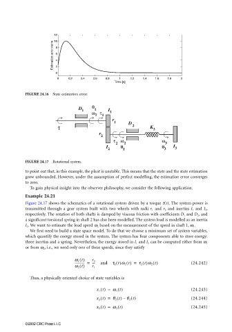
FIGURE 24.16 State estimation error.
θ
D 1
1 I
ω 1 τ 1 1
r
1 D
τ 2 K 2
r
2
τ ω ω
2 2 3
I θ θ I 3
2 2 3

FIGURE 24.17 Rotational system.
to point out that, in this example, the plant is unstable. This means that the state and the state estimation
grow unbounded. However, under the assumption of perfect modelling, the estimation error converges
to zero.
To gain physical insight into the observer philosophy, we consider the following application.
Example 24.21
Figure 24.17 shows the schematics of a rotational system driven by a torque t(t). The system power is
transmitted through a gear system built with two wheels with radii r 1 and r 2 and inertias I 1 and I 2 ,
respectively. The rotation of both shafts is damped by viscous friction with coefficients D 1 and D 2 , and
a significant torsional spring in shaft 2 has also been modelled. The system load is modelled as an inertia
I 3 . We want to estimate the load speed w 3 based on the measurement of the speed in shaft 1, w 1 .
We first need to build a state space model. To do that we choose a minimum set of system variables,
which quantify the energy stored in the system. The system has four components able to store energy:
three inertias and a spring. Nevertheless, the energy stored in I 1 and I 2 can be computed either from w 1
or from w 2 , i.e., we need only one of these speeds, since they satisfy

w 1 t()
------------- = r 2 and t 1 t()w 1 t() = t 2 t()w 2 t() (24.242)
----
w 2 t() r 1
Thus, a physically oriented choice of state variables is

x 1 t() = w 1 t() (24.243)
x 2 t() = q 2 t() q 3 t() (24.244)
–
x 3 t() = w 3 t() (24.245)

©2002 CRC Press LLC