Page 797 - The Mechatronics Handbook

0066_Frame_C24 Page 45 Thursday, January 10, 2002 3:46 PM

40
20 ω
|H (j )|
2
Magnitude [dB] -20 0
ω
|H (j )|
-40 1
-60
10 -1 10 0 10 1 10 2 10 3
Frequency [rad/s]

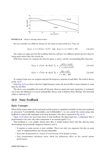
FIGURE 24.18 Observer filtering characteristics.
We next consider two different choices for the observer polynomial E(s). They are

E 1 s() = ( s + 0.5) s + 0.75) and E 2 s() = ( s + 10) s + 20) (24.262)
(
(
The reader can appreciate that the resulting observers will have very different speeds, the first observer
being much slower than the second one.
With those choices we compute the observer gains, J 1 and J 2 , and the corresponding filter functions

1.875s + 5.625
T
H 1 s() = g sIA + J 1 C) J 1 = ----------------------------------------- (24.263)
1
–
(
–
s + 1.25s + 0.375
2
144s + 432
(
H 2 s() = g sIA + J 2 C) J 2 = --------------------------------- (24.264)
T
1
–
–
s + 30s + 200
2
To compare both cases we compute and plot the frequency response of each filter. The result is shown
in Fig. 24.18.
From Fig. 24.18 we observe that for a high frequency noise, the slowest filter is more immune to noise
than the fast filter.
The above case exemplifies the trade-off between observer speed and noise immunity. A systematic
way to face this dilemma is to use an optimal filter theory, such as Kalman–Bucy filtering. The interested
reader is referred to [2].
24.8 State Feedback
Basic Concepts
When all the system states can be measured, and the system is completely reachable (in the sense explained
in subsection “Controllability, Reactability, and Stabilizability”), we can control the system using state
feedback to achieve full command of the loop dynamics. This idea is captured in Fig. 24.19.
Figure 24.19 shows the most basic form of state feedback: the plant input has a component that is
r
proportional to the state (the other component is an external signal (t)).
State feedback is a very simple, almost naive idea. A careful analysis shows that this idea has some
shortcomings and potentially dangerous features, such as

• It requires as many sensors as state variables. This is not only very expensive but also, in some
cases, its implementation may become impossible.
• Each state measurement is a source of error because of its limited accuracy.
• Each measurement introduces noise, which has deleterious effect on the control system
performance.

©2002 CRC Press LLC