Page 803 - The Mechatronics Handbook

0066_Frame_C25 Page 2 Wednesday, January 9, 2002 7:05 PM

j
j
in which a linear combination is taken using the jth order time derivatives d /dt of a single output y(t)
≠ 0 and b j for j =
and a single input u(t). In (25.1), the scalar real valued numbers a j for j = 0,…n a , a n
a
≠ 0, respectively, are called the denominator and numerator coefficients. The input u(t) is
0,…,n b , b n
b
distinguished from the output y(t) in (25.1) by requiring n a ≥ n b . As a result, the n a th derivative is the
highest derivative of the output y(t) and n a is used to indicate the order of the differential equation.
An alternative representation of a model of a continuous time system can be obtained by rewriting the
n a th order differential equation in (25.1) into a set of (coupled) first order differential equations. This can
be done by introducing a state variable x(t) and rewriting the higher order differential equation into
d
-----xt() = Ax t() + Bu t()
dt (25.2)
yt() = Cx t() + Du t()

where A, B, C, and D are real valued matrices. The set of first order differential equations given in (25.2)
is referred to as a state space representation. The state variable x(t) is a column vector and contains n a
variables, where n a is the order of the differential equation.
The size of the matrices in (25.2) corresponds to the order of differential equation from which the
state space realization is derived. For generalization purposes, consider multiple inputs and outputs
rearranged in m × 1 input column vector u(t) and a p × 1 output column vector y(t). Given the n a × 1
size of the state vector, the state matrix A has size n a × n a , the input matrix has size n a × m, the output
matrix C has size p × n a , and the feedthrough matrix D has size m × p. From these size considerations
it can be observed that the state space realization in (25.2) easily generalizes the model description of
multi-input multi-output systems.
To illustrate the concepts, consider the differential equation

2
d
d
m -------yt() + c----- yt() + ky t() = ut() (25.3)
dt 2 dt
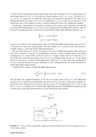
that describes the dynamical behavior of the one cart system given in Fig. 25.1. The differential
equation (25.3) is found by writing Newton’s second law for the cart mass m with position output y(t),
spring force ky(t), damper force c(d/dt)y(t), and force input u(t). Comparing with (25.1) it can be seen
that n a = 2 ≥ n b = 0, making (25.3) a second order differential equation. The differential equation can be
rewritten into a state space representation (25.2) by defining the state variable

yt()
xt() :=
d
----- yt()
dt

FIGURE 25.1 One cart system representing a single mass dynamical system with cart mass m, spring constant k,
and damping constant c.

©2002 CRC Press LLC