Page 772 - The Mechatronics Handbook

0066_Frame_C24 Page 20 Thursday, January 10, 2002 3:44 PM

1
0.8
0.6
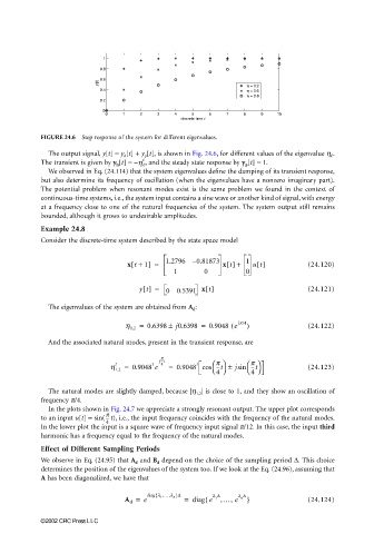
y[t] η = 0.2
0.4 η = 0.6
η = 0.8
0.2
0
0 1 2 3 4 5 6 7 8 9 10
discrete time t
FIGURE 24.6 Step response of the system for different eigenvalues.

The output signal, y[t] = y h [t] + y p [t], is shown in Fig. 24.6, for different values of the eigenvalue h .
t
The transient is given by y h [t] = −h , and the steady state response by y p [t] = 1.
We observed in Eq. (24.114) that the system eigenvalues define the damping of its transient response,
but also determine its frequency of oscillation (when the eigenvalues have a nonzero imaginary part).
The potential problem when resonant modes exist is the same problem we found in the context of
continuous-time systems, i.e., the system input contains a sine wave or another kind of signal, with energy
at a frequency close to one of the natural frequencies of the system. The system output still remains
bounded, although it grows to undesirable amplitudes.
Example 24.8
Consider the discrete-time system described by the state space model

x t + 1] = 1.2796 – 0.81873 x t[] + 1 ut[] (24.120)
[
1 0 0
yt[] = 0 0.5391 x t[] (24.121)

The eigenvalues of the system are obtained from A d :
(
h 1,2 = 0.6398 ± j0.6398 = 0.9048 e jp/4 ) (24.122)

And the associated natural modes, present in the transient response, are
p
j---t  
p
p
t
t
t
h 1,2 = 0.9048 e 4 = 0.9048 cos ---t ± jsin ---t (24.123)
4  4 
The natural modes are slightly damped, because |h 1,2 | is close to 1, and they show an oscillation of
frequency p/4.
In the plots shown in Fig. 24.7 we appreciate a strongly resonant output. The upper plot corresponds
p
to an input u[t] = sin( t), i.e., the input frequency coincides with the frequency of the natural modes.
---
4
In the lower plot the input is a square wave of frequency input signal p/12. In this case, the input third
harmonic has a frequency equal to the frequency of the natural modes.
Effect of Different Sampling Periods
We observe in Eq. (24.95) that A d and B d depend on the choice of the sampling period ∆. This choice
determines the position of the eigenvalues of the system too. If we look at the Eq. (24.96), assuming that
A has been diagonalized, we have that
{
A d = e diag l ,…,l }∆ = diag e l ∆ ,…, e l ∆ } (24.124)
{
1
n
1
n
©2002 CRC Press LLC