Page 766 - The Mechatronics Handbook

0066_Frame_C24 Page 14 Thursday, January 10, 2002 3:44 PM

Now choose as state variables,

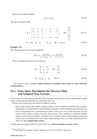
x (t) = v (t) (24.76)

The above equations yield

0
0 1 0 ⋅⋅⋅ 0 0 0
A = 0 0 1 ⋅⋅⋅ 0 0 , B = (24.77)

0
– a 0 – a 1 – a 2 ⋅⋅⋅ – a n−2 – a n−1
1
C = [ b 0 b 1 b 2 … b n−1 ], D = H T ∞() (24.78)

Example 24.5
The transfer function of a system is given by

–
4s 10 4s 10
–
Hs() = ---------------------------------- = -------------------------- (24.79)
2
( s + 2) s 1–( ) s + 3s – 4
3
2
Then a minimal realization for this system is
01 0 0
A = 00 1 , B = 0 (24.80)
40 – 3 1

C = – 10 40 , D = 0 (24.81)

A key result is that a system transfer function is invariant with respect to state similarity
transformations.

24.4 State Space Description for Discrete-Time
and Sampled Data Systems

In this section we will present an overview of the state space description for discrete time systems, mainly
based on the results presented for the continuous time case.
Discrete time models may arise from two different sources:
• From a pure discrete-time system, usually nonlinear, whose variables are defined only at specific
time instants t k . Systems like that can be found in economic systems, stochastic process theory, etc.
• From a discretization of a continuous-time system. In this case, we are only concerned with the
value of some system variables at specific time instants. These models are useful when digital
systems, such as microcontrollers, computers, PLCs, or others, interact with continuous-time real
1
systems such as mechanical structures, valves, tanks, analog circuits or a whole industrial process .
These are called sampled data systems.
In both cases our analysis will be focused on the class of linear and time invariant models.

1
Through digital-to-analog and analog-to-digital converters (DAC and ADC, respectively).

©2002 CRC Press LLC