Page 764 - The Mechatronics Handbook

0066_Frame_C24 Page 12 Thursday, January 10, 2002 3:44 PM

T
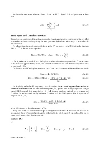
An alternative state vector is x t() = [ x 1 t() x 2 t()] = [ it() i 2 t()] T . It is straightforward to show
that

1
1 R 2
x t() = ----- x t() (24.63)
1
R 2 0
    
T
State Space and Transfer Functions

The state space description of linear time invariant systems is an alternative description to that provided
by transfer functions. Strictly speaking, the state space description has a wider scope, as we shall see in
this subsection.
p
m
For a linear time invariant system with input u(t) and output y(t) , the transfer function,
H(s) C p ×m , is defined by the equation
Y i s()
Y s() = H s()U s(), where [ H s()] ij = ------------ (24.64)
U j s()

th
i.e., the (i, j) element in matrix H(s) is the Laplace transformation of the response in the i output when
th
a unit impulse is applied at the j input, with zero initial conditions and with the remaining inputs equal
to zero for all t ≥ 0.
On the other hand, if we Laplace-transform (24.42) and (24.43) with zero initial conditions, we obtain

–
X s() = ( sIA) BU s() (24.65)
1
–
Y s() = CX s() + DU s() = ( C sIA) B + D) U s() (24.66)
1
–
(
–
        
H s()
For simplicity, and to be able to go deeper into the analysis, in the remaining part of this section we
will focus our attention on the class of scalar systems, i.e., systems with a single input and a single
output (SISO systems). This means that m = p = 1, B becomes a column vector, C is a row vector, and
D = H(∞) (in real systems it usually holds that D = H(∞) = 0). For SISO systems, H(s) is a quotient of
polynomials in s, i.e.,
(
(
C Adj sIA)B + D det sIA)
–
–
Hs() = ---------------------------------------------------------------------------- (24.67)
(
det sIA)
–
where Adj(o) denotes the adjoint matrix of (o).
A key issue is that the transfer function poles are eigenvalues of matrix A. However, it is not true, in
general, that the set of transfer function poles is identical to the set of matrix A eigenvalues. This can be
appreciated through the following example.
Example 24.4
Let

A = – 2 1 , B = 1 , C = 0 1 , D = 0 (24.68)
0 – 3 0.5

©2002 CRC Press LLC