Page 868 - The Mechatronics Handbook

0066_Frame_C28 Page 8 Wednesday, January 9, 2002 7:19 PM

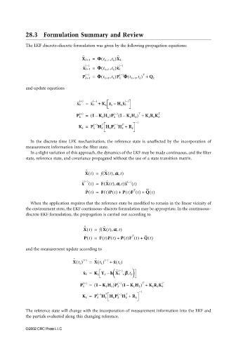
28.3 Formulation Summary and Review

The LKF discrete–discrete formulation was given by the following propagation equations:

˜ ˜
(
X k+1 = ΦΦ Φ Φ t k+1 ,t k )X k
− () − ()
(
x ˆ k+1 = ΦΦ Φ Φ t k+1 ,t k )x ˆ k
− ()
− ()
(
P k+1 = ΦΦ Φ Φ t k+1 ,t k )P k ΦΦ ΦΦ t k+1 ,t k ) + Q k
T
(
and update equations
+ () − () − ()
x ˆ k = x ˆ k + K k z k – H k x ˆ k
− ()
+ () = ( IK k H k )P k ( IK k H k ) + T
T
P k – – K k R k K k
−1
− () T − () T
K k = P k H k H k P k H k + R k
In the discrete time LFK mechanization, the reference state is unaffected by the incorporation of
measurement information into the filter state.
In a slight variation of this approach, the dynamics of the LKF may be made continuous, and the filter
state, reference state, and covariance propagated without the use of a state transition matrix.

˜ ˙
˜
(
X t() = f X t(),αα αα, t)
˜
(
˙ x ˆ − () t () = FX t(),αα αα,t)x ˆ − () t ()
˙
T
P t() = F t()P t() + P t()F t() + Q t()
When the application requires that the reference state be modified to remain in the linear vicinity of
the environment state, the EKF continuous–discrete formulation may be appropriate. In the continuous–
discrete EKF formulation, the propagation is carried out according to
˜ ˙ ˜
(
X t() = f X t(),αα αα, t)
˙
T
P t() = F t()P t() + P t()F t() + Q t()
and the measurement update according to

˜ () + () = ˜ () − () + ()
X t k X t k x ˆ t k
˜ 
− ()
x ˆ k = K k Y k – h X k ,ββ ββ,t k  

+ () = ( IK k H k )P k ( IK k H k ) + T
− ()
T
P k – – K k R k K k
−1
− () T − () T
K k = P k H k H k P k H k + R k
The reference state will change with the incorporation of measurement information into the EKF and
the partials evaluated along this changing reference.

©2002 CRC Press LLC