Page 863 - The Mechatronics Handbook

0066_Frame_C28 Page 3 Wednesday, January 9, 2002 7:19 PM

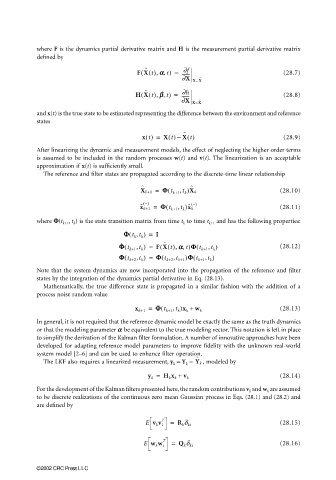
where F is the dynamics partial derivative matrix and H is the measurement partial derivative matrix
defined by

∂f
FX t(), αα αα, t( ˜ ) = ------- (28.7)
∂X X=X ˜
˜
HX t(), ββ ββ, t) = ------- (28.8)
(
∂h
∂X X=X ˜
and x(t) is the true state to be estimated representing the difference between the environment and reference
states
˜
–
x t() = X t() X t() (28.9)
After linearizing the dynamic and measurement models, the effect of neglecting the higher order terms
is assumed to be included in the random processes w(t) and v(t). The linearization is an acceptable
approximation if x(t) is sufficiently small.
The reference and filter states are propagated according to the discrete-time linear relationship

˜ ˜
(
X k+1 = ΦΦ Φ Φ t k+1 ,t k )X k (28.10)
− () − ()
(
x ˆ k+1 = ΦΦ Φ Φ t k+1 ,t k )x ˆ k (28.11)
where ΦΦ ΦΦ(t k+1 , t k ) is the state transition matrix from time t k to time t k+1 and has the following properties:
(
ΦΦ Φ Φ t k ,t k ) = I
˜
(
(
ΦΦ Φ Φ ˙ ( t k+1 ,t k ) = FX t(), αα αα, t)ΦΦ ΦΦ t k+1 ,t k ) (28.12)
ΦΦ Φ Φ t k+2 ,t k ) = ΦΦ Φ Φ t k+2 ,t k+1 )ΦΦ ΦΦ t k+1 ,t k )
(
(
(
Note that the system dynamics are now incorporated into the propagation of the reference and filter
states by the integration of the dynamics partial derivative in Eq. (28.13).
Mathematically, the true difference state is propagated in a similar fashion with the addition of a
process noise random value
(
x k+1 = ΦΦ Φ Φ t k+1 ,t k )x k + w k (28.13)
In general, it is not required that the reference dynamic model be exactly the same as the truth dynamics
or that the modeling parameter αα αα be equivalent to the true modeling vector. This notation is left in place
to simplify the derivation of the Kalman filter formulation. A number of innovative approaches have been
developed for adapting reference model parameters to improve fidelity with the unknown real-world
system model [2–6] and can be used to enhance filter operation.
˜
The LKF also requires a linearized measurement, y k = Y k − Y k , modeled by
y k = H k x k + v k (28.14)

For the development of the Kalman filters presented here, the random contributions v k and w k are assumed
to be discrete realizations of the continuous zero mean Gaussian process in Eqs. (28.1) and (28.2) and
are defined by

T =
E v k v i R k d ki (28.15)

T =
E w k w i Q k d ki (28.16)

©2002 CRC Press LLC