Page 862 - The Mechatronics Handbook

0066_Frame_C28 Page 2 Wednesday, January 9, 2002 7:19 PM

Reference Trajectory

State Estimate

True Trajectory

Estimation Error
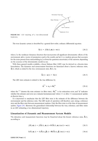
FIGURE 28.1 LKF tracking of a two-dimensional
trajectory.

The true dynamic system is described by a general first-order, ordinary differential equation

X t() = f X t(),αα αα,t) + w t() (28.2)
˙
(
where f is the nonlinear dynamics function that incorporates all significant deterministic effects of the
environment, αα αα is a vector of parameters used in the model, and w(t) is a random process that accounts
for the noise present from mismodeling in f or from the quantum uncertainty of the universe, depending
on the accuracy of the deterministic model in use.
With these general models available, a linear Kalman filter (LKF) may be derived in a discrete-time
formulation. The dynamics and measurement functions are linearized about a known reference state,
˜
X (t), which is related to the true environment state, X(t), via

˜
X t() + x t() = X t() (28.3)

The LKF state estimate is related to the true difference by

± () ± ()
x ˆ k = x k + dx k (28.4)

± ()
ˆ is the estimation error, and “±” indicates

where the “” denotes the state estimate (or filter state), dx k
whether the estimate and error are evaluated instantaneously before (−) or after (+) measurement update
at discrete time t k .
It is important to emphasize that the LKF filter state is the estimate of the difference between the
environment and the reference state. The LKF mode of operation will therefore carry along a reference
state and the filter state between measurement updates. Only the filter state is at the time of measurement
update. Figure 28.1 illustrates the generalized relationship between the true, reference, and filter states
in an LKF estimating a two-dimensional trajectory.

Linearization of Dynamic and Measurement System Models
˜
X
The dynamics and measurement functions may be linearized about the known reference state, (t),
according to
˜
˜
f X, αα αα, t( ) f X t(), αα αα, t) + FX t(), αα αα, t)x t() + w t() (28.5)
(
(
˜
˜
h X, αα αα, t( ) h X t(), ββ ββ, t) + HX t(), ββ ββ, t)x t() + v t() (28.6)
(
(
©2002 CRC Press LLC