Page 873 - The Mechatronics Handbook

0066-frame-C29 Page 3 Wednesday, January 9, 2002 7:23 PM

While the DTFT is continuous with respect to the frequency variable Ω, the discrete Fourier transform
(DFT) contains points that are discrete with respect to a parameter k. Consider a finite duration sequence
x[n], where x[n] = 0 for n < 0 and for n ≥ N. The DFT of x[n] and the inverse DFT are defined as

N−1
X k ∑ xn[]e −j2pnk/N , k = 0, 1,…, N 1 (29.4)
=
–
n=0
and

N−1
1
x n = ---- ∑ X k e j2pnk/N , n = 0, 1,…, N 1
–
N
k=0
over the range Ω = 0
Note that the DFT is a discretized version of the DTFT where X k = X(Ω)| Ω=2pk/N
to Ω = 2π. Calculating a closed-form solution for the DTFT can be done only for simple signals such as
a square pulse or a triangular pulse. Therefore, the DFT is generally used as a numerical method to
calculate the DTFT at discrete points in frequency in the range 0 ≤ Ω ≤ 2π. In particular, to obtain a plot
of the DTFT, plot X k versus k where k is scaled by 2π/N. For an arbitrary signal, such as obtained from
measurements of a physical device, computing the DFT instead of the DTFT is the preferred method to
find the frequency content of the signal. To get more resolution in plotting a DTFT from the points
calculated by a DFT, zeros can be added to the end of the sequence so that the value of N is increased.
Suppose a time domain signal is not finite in duration, so that there is no value of N such that x[n] = 0
for n ≥ N. In order to perform the DFT, the signal must be truncated. There are two cases to be considered:
the case where x[n] is decaying to zero and the case where x[n] has periodic components. The case when
x[n] decays to zero is handled by choosing N to be large enough so that the signal is negligible beyond
that value. The resulting DFT is an approximation (not a discretized version) of the DTFT. If the signal
is periodic, the DTFT cannot be computed numerically since the resulting DTFT would have impulses
in it. However, the frequencies present in the signal could still be determined if the value of N used for
the truncation is chosen so that the truncated signal goes through an integer number of cycles. If this
not done, the resulting DFT will have leakage in the frequency plot when compared to the DTFT of the
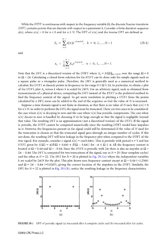
true signal. For example, consider a signal x[n] = cos(0.4πn). This is periodic with period n = 5 and has
DTFT given by X(Ω) = π[δ(Ω + 0.4π) + δ(Ω − 0.4π)] for −π ≤ Ω ≤ π. All the frequency content is
located at Ω = 0.4p and Ω = −0.4π. Since the DTFT is periodic with 2π, there is also an impulse at Ω =
2π − 0.4π. The DFT is computed for two truncations of the signal, one at N = 20 (four complete cycles)
and the other at N = 22. The DFT for N = 20 is plotted in Fig. 29.1(a) where the independent variables
k are scaled by 2π/N for the plot. This plot shows zero frequency content except at Ω = 0.4π (=1.2566)
and Ω = 2π − 0.4π (=5.0265), giving the correct location of the impulses in the DTFT. Similarly, the
DFT for N = 22 is plotted in Fig. 29.1(b), notice the resulting leakage in the frequency characteristics.

15 15

10 10
|X(Ω)| |X(Ω)|
5 5

0 0
0 2 4 6 0 2 4 6
Ω Ω
(a) (b)

FIGURE 29.1 DFT of periodic signal (a) truncated after 4 complete cycles and (b) truncated after 4.4 cycles.

©2002 CRC Press LLC