Page 895 - The Mechatronics Handbook

0066_Frame_C30 Page 6 Thursday, January 10, 2002 4:43 PM

Closed Loop Transfer Function Matrices
Given the structure for the generalized plant G, we have the following closed loop relationships:

u = Ky (30.14)
(
= KG 21 w + G 22 u) (30.15)
–
1
–
= [ IKG 22 ] KG 21 w (30.16)
–
1
= KI G 22 K–[ ] G 21 w (30.17)
–
1
y = [ I G 22 K] G 21 w (30.18)
–
z = G 11 w + G 12 u (30.19)
= G 11 w + G 12 Ky (30.20)
–
1
[
–
= [ G 11 + G 12 KI G 22 K] G 21 ]w (30.21)
From this, we have the following closed loop transfer function matrices:
[
1
–
–
T wu = KI G 22 K] G 21 (30.22)
–
1
–
T wy = [ IG 22 K] G 21 (30.23)
[
1
–
–
T wz = G 11 + G 12 KI G 22 K] G 21 (30.24)
We say that each of these is a linear fractional transformation (LFT) involving K.
Comment 30.8 (Well Posedness of Closed Loop System)
−l
In the above manipulation, it has been assumed that the inverse [I − G 22 K] is well defined. This well
posedness condition is guaranteed by our assumption that D 22 = 0. This assumption implies that G 22 (j∞) =
D 22 = 0 and hence that the inverse is well defined.
3
The following example shows how to formulate a so-called Weighted H Mixed Sensitivity Problem
to address feedback control system design issues.
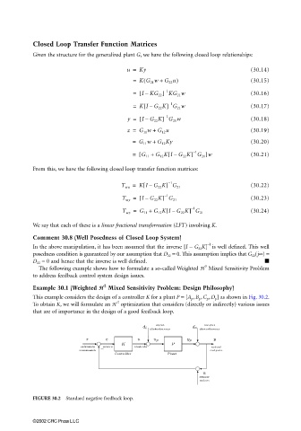
Example 30.1 (Weighted HH 2 Mixed Sensitivity Problem: Design Philosophy)
This example considers the design of a controller K for a plant P = [A p , B p , C p , D p ] as shown in Fig. 30.2.
2
To obtain K, we will formulate an H optimization that considers (directly or indirectly) various issues
that are of importance in the design of a good feedback loop.

FIGURE 30.2 Standard negative feedback loop.

©2002 CRC Press LLC