Page 288 - Thomson, William Tyrrell-Theory of Vibration with Applications-Taylor _ Francis (2010)

Sec. 9.3 Torsional Vibration of Rods 275

The natural frequencies of the bar hence are determined by the equation
( 1 \ 7T / G

“ ” I + 2 ) J \ J
where n = 0,1,2,3,... .
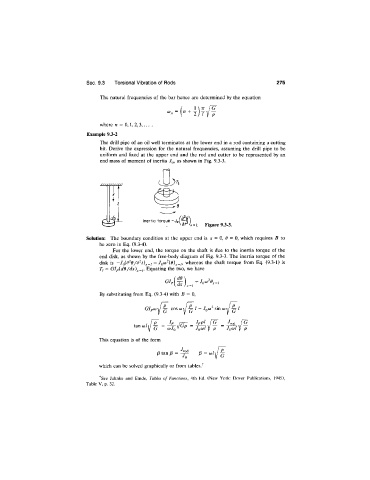
Example 9.3-2
The drill pipe of an oil well terminates at the lower end in a rod containing a cutting
bit. Derive the expression for the natural frequencies, assuming the drill pipe to be
uniform and iked at the upper end and the rod and cutter to be represented by an
end mass of moment of inertia Jq, as shown in Fig. 9.3-3.

Figure 9.3-3.

Solution: The boundary condition at the upper end is jc = 0, 0 = 0, which requires B to
be zero in Eq. (9.3-4).
For the lower end, the torque on the shaft is due to the inertia torque of the
end disk, as shown by the free-body diagram of Fig. 9.3-3. The inertia torque of the
disk is = Jq(x)^{6)^^i, whereas the shaft torque from Eq. (9.3-1) is
7) = GIp(dd/dx)^^i. Equating the two, we have

By substituting from Eq. (9.3-4) with B = 0,

Gipcoy cos ioy -pr / = sin it)-» / -pr /

I / P
.
ta n (x)l\l ^ — (o J q ^ rF~ — ^PP^ 1 \i J q(x)1 I
T
T
T y ( j p
G
J q(o i y p
This equation is of the form
p i a n p = ~ Y ^ p = w l
•'0
which can be solved graphically or from tables.^
^See Jahnke and Emde, Tables of Functions, 4th Ed. (New York: Dover Publications, 1945),
Table V, p. 32.