Page 292 - Thomson, William Tyrrell-Theory of Vibration with Applications-Taylor _ Francis (2010)

Sec. 9.4 Vibration of Suspension Bridges 279

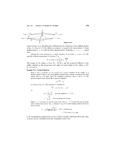
Figure 9.4-3.
shown in Fig. 9.4-3. Recalling the definition for the elements of the stiffness matrix
in Sec. 6.3, Eq. (6.3-1), the stiffness at station i is equal to the lateral force F when

displacement == 1.0 with all other displacements, including y^_j, y-^j,..., equal
zero.
Giving the cross section at i a small rotation, 0, we have y- = x4> = {b/2)6,
and the vertical component of tension T is
F = 2T4> = 2 T ^ 8 = ^

The torque of the cables is then Fb = Tb^d/x and the torsional stiffness of the
cables, defined as the torque per unit angle per unit length of the cables, is Tb^
lb • ft/rad/ft.
Example 9.4-1 Vertical Vibration
With T and p constant, we can analyze the vertical vibration of the bridge as a
flexible string of mass p per unit length stretched under tension T between two rigid
towers that are / ft apart. With the boundary conditions y(0,/) = y(/, t) = 0, the
general solution must satisfy the frequency equation
. col _
sm — = 0
c
as shown in Sec. 9.1. This equation is satisfied by
col
= 77,2 t7 , 377, .
c
or
n [T
fn = 21 1 p , Ai(mode number) = 1,2,3,.
/
T
= wave propagation velocity
When /I = 1, we have the fundamental mode; when /i = 2, we have the second mode
with a node at the center; etc., as shown in Fig. 9.4-4. Substituting numbers from the
data, we have
/ 13.1
fn = 2 X 2800 V 96.4 X lO'’ - 0.0658A7 cps
= 3.95/1 cpm = An cpm

F. B. Farquharson reported that several different modes had been observed, some
of which can be identified with the computed results here.