Page 43 - Thomson, William Tyrrell-Theory of Vibration with Applications-Taylor _ Francis (2010)

30 Free Vibration Chap. 2

and we can also express 2 terms of ^ as follows:

2m 2m )
Equation (2.6-6) then becomes
il,2 = (-C ± - 1 (2.6-11)

The three cases of damping discussed here now depend on whether is
greater than, less than, or equal to unity. Furthermore, the differential equation of
motion can now be expressed in terms of ^ and as
X + 2Cù)„x + U)lx = ^ P ( t) ( 2.6-12)

This form of the equation for single-DOF systems will be found to be helpful in
identifying the natural frequency and the damping of the system. We will fre­
quently encounter this equation in the modal summation for multi-DOF systems.
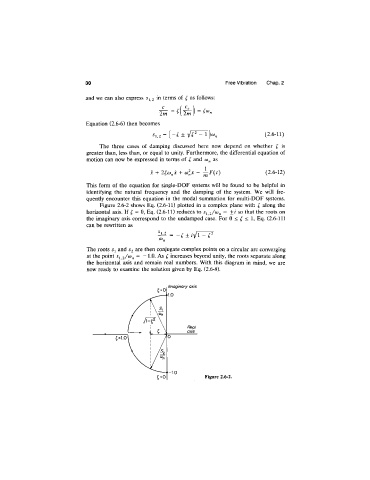
Figure 2.6-2 shows Eq. (2.6-11) plotted in a complex plane with along the
horizontal axis. If ^ = 0, Eq. (2.6-11) reduces to s^ 2/^n = so that the roots on
the imaginary axis correspond to the undamped case. For 0 < ^ < 1, Eq. (2.6-11)
can be rewritten as

The roots and ^2 then conjugate complex points on a circular arc converging
at the point “ l-O- As increases beyond unity, the roots separate along
the horizontal axis and remain real numbers. With this diagram in mind, we are
now ready to examine the solution given by Eq. (2.6-8).

Figure 2.6-2.