Page 489 - Thomson, William Tyrrell-Theory of Vibration with Applications-Taylor _ Francis (2010)

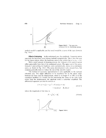
476 Nonlinear Vibrations Chap. 14

Figure 14.6-3. The jump phe­
nomenon for the hardening spring.
analysis would be applicable and the result would be a curve of the type shown in
Fig. 14.6-3.

Effect of damping. In the undamped case, the amplitude-frequency curves
approach the backbone curve (shown dashed) asymptotically. This is also the case
for the linear system, where the backbone curve is the vertical line at (o/co^^ = 1.0.
With a small amount of damping present, the behavior of the system cannot
differ appreciably from that of the undamped system. The upper end of the curve,
instead of approaching the backbone curve asymptotically, crosses in a continuous
curve, as shown in Fig. 14.6-4. The jump phenomenon is also present here, but
damping generally tends to reduce the size of the unstable region.
The method of successive approximation is also applicable to the damped
vibration case. The major difference in its treatment lies in the phase angle
between the force and the displacement, which is no longer 0° or 180° as in the
undamped problem. It is found that by introducing the phase in the force term
rather than the displacement, the algebraic work is somewhat simplified. The
differential equation can then be written as
X + cx + iJiX^ = F cos (ojt F (f))
(14.6-7)
= cos (i)t — sin cot
where the magnitude of the force is

F= yjAl + (14.6-8)

Figure 14.6-4.