Page 161 - Bird R.B. Transport phenomena

Problems 145
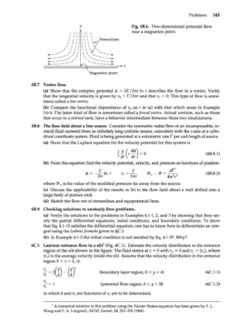
Fig. 4B.6. Two-dimensional potential flow
near a stagnation point.
/ / I I M i l
/ / I I
/ / I I им
/ I I I I 1 \ \ Streamlines
/ I I I I I \
/ I I I I \ \
' I I \ \ \
' ' ' I \ \
/
Stagnation point

4B.7 Vortex flow.
(a) Show that the complex potential zv = (iY/lir) In z describes the flow in a vortex. Verify
that the tangential velocity is given by v 0 = Г/2тгг and that v r = 0. This type of flow is some-
times called a free vortex.
(b) Compare the functional dependence of v e on r in (a) with that which arose in Example
3.6-4. The latter kind of flow is sometimes called a forced vortex. Actual vortices, such as those
that occur in a stirred tank, have a behavior intermediate between these two idealizations.

4B.8 The flow field about a line source. Consider the symmetric radial flow of an incompressible, in-
viscid fluid outward from an infinitely long uniform source, coincident with the z-axis of a cylin-
drical coordinate system. Fluid is being generated at a volumetric rate Г per unit length of source.
(a) Show that the Laplace equation for the velocity potential for this system is

T('T) 0 (4B 8 1)
- -
dr \ dr )
(b) From this equation find the velocity potential, velocity, and pressure as functions of position:
Ф = ~ In r v r = ^- P, - P = -^j-z (4B.8-2)
2тг 2irr S 2 2
<
>
where 3 is the value of the modified pressure far away from the source.
x
(c) Discuss the applicability of the results in (b) to the flow field about a well drilled into a
large body of porous rock.
(d) Sketch the flow net of streamlines and equipotential lines.
4B.9 Checking solutions to unsteady flow problems.
(a) Verify the solutions to the problems in Examples 4.1-1, 2, and 3 by showing that they sat-
isfy the partial differential equations, initial conditions, and boundary conditions. To show
that Eq. 4.1-15 satisfies the differential equation, one has to know how to differentiate an inte-
gral using the Leibniz formula given in §C3.
(b) In Example 4.1-3 the initial condition is not satisfied by Eq. 4.1-57. Why?
4C.1 Laminar entrance flow in a slit 3 (Fig. 4C.1). Estimate the velocity distribution in the entrance
region of the slit shown in the figure. The fluid enters at x = 0 with v = 0 and v = (v ), where
y x x
(v ) is the average velocity inside the slit. Assume that the velocity distribution in the entrance
x
region 0 < x < L is
c
v (y\ (y\ 2
x
-^ = 2l ^ J - I ^ I (boundary layer region, 0 < у < 8) (4C.1-1)
-£ = 1 (potential flow region, 8 < у < В) (4С.1-2)
in which 8 and v are functions of x, yet to be determined.
c
3 A numerical solution to this problem using the Navier-Stokes equation has been given by Y. L.
Wang and P. A. Longwell, AIChE Journal, 10, 323-329 (1964).