Page 156 - Bird R.B. Transport phenomena

140 Chapter 4 Velocity Distributions with More Than One Independent Variable

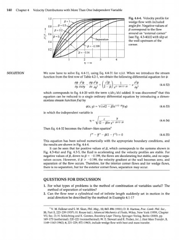
1.0 Fig. 4.4-4. Velocity profile for
wedge flow with included
0.8 angle /Зтг. Negative values of
/3 correspond to the flow
0.6 around an "external corner"
[see Fig. 4.3-4Ш)] with slip at
0.4 the wall upstream of the
corner.
0.2

SOLUTION We now have to solve Eq. 4.4-11, using Eq. 4.4-31 for v (x). When we introduce the stream
e
function from the first row of Table 4.2-1, we obtain the following differential equation for ф:
г
дф д ф дф д ф _ I с р ^ 1 д ф
2
3
2
(4.4-32)
~fry~dx~dy~~dx~rf~\2-p
which corresponds to Eq. 4.4-20 with the term v (dv /dx) added. It was discovered 9 that this
e
e
equation can be reduced to a single ordinary differential equation by introducing a dimen-
sionless stream function f(rj) by
ф(х,у) = (4.4-33)
in which the independent variable is
У
(4.4-34)
Then Eq. 4.4-32 becomes the Falkner-Skan equation 9
2
f'"-ff"-p(\ -/' ) = (4.4-35)
This equation has been solved numerically with the appropriate boundary conditions, and
the results are shown in Fig. 4.4-4.
It can be seen that for positive values of /3, which corresponds to the systems shown in
Fig. 4.3-4(a) and Fig. 4.3-5, the fluid is accelerating and the velocity profiles are stable. For
negative values of j3, down to /3 = -0.199, the flows are decelerating but stable, and no sepa-
ration occurs. However, if /3 > -0.199, the velocity gradient at the wall becomes zero, and
separation of the flow occurs. Therefore, for the interior corner flows and for wedge flows,
there is no separation, but for the exterior corner flows, separation may occur.

QUESTIONS FOR DISCUSSION

1. For what types of problems is the method of combination of variables useful? The
method of separation of variables?
2. Can the flow near a cylindrical rod of infinite length suddenly set in motion in the
axial direction be described by the method in Example 4.1-1?

9
V. M. Falkner and S. W. Skan, Phil. Mag., 12, 865-896 (1931); D. R. Hartree, Proc. Camb. Phil. Soc,
33, Part II, 223-239 (1937); H. Rouse (ed.), Advanced Mechanics of Fluids, Wiley, New York (1959), Chapter
VII, Sec. D; H. Schlichting and K. Gersten, Boundary-Layer Theory, Springer-Verlag, Berlin (2000), pp.
169-173 (isothermal), 220-221 (nonisothermal); W. E. Stewart and R. Prober, Int. J. Heat Mass Transfer, 5,
1149-1163 (1962); 6, 221-229, 872 (1963), include wedge flow with heat and mass transfer.