
Page 155 - Bird R.B. Transport phenomena
P. 155
§4.4 Flow near Solid Surfaces by Boundary-Layer Theory 139
1.0
0.8 /
0.6
X
R
0.4
+ 1.08x1o 5
* 1.82x1o 5
o3.64x1o 5
0.2 • ^.46x1n 5
Д .28x1o 5
7
/
/
1.0 2.0 3.0 4.0 5.0 5.64 6.0 7.0
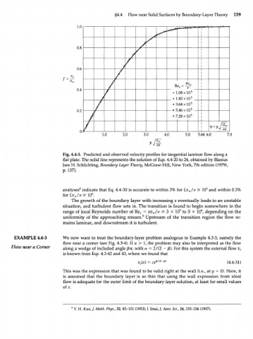
Fig. 4.4-3. Predicted and observed velocity profiles for tangential laminar flow along a
flat plate. The solid line represents the solution of Eqs. 4.4-20 to 24, obtained by Blasius
[see H. Schlichting, Boundary-Layer Theory, McGraw-Hill, New York, 7th edition (1979),
p. 137].
4
analyses 8 indicate that Eq. 4.4-30 is accurate to within 3% for Lv /v > 10 and within 0.3%
x
iorLv /v> 10. 6
x
The growth of the boundary layer with increasing x eventually leads to an unstable
situation, and turbulent flow sets in. The transition is found to begin somewhere in the
6
5
range of local Reynolds number of Re v = xv /v > 3 X 10 to 3 X 10 , depending on the
x
uniformity of the approaching stream. 8 Upstream of the transition region the flow re-
mains laminar, and downstream it is turbulent.
EXAMPLE 4.4-3 We now want to treat the boundary-layer problem analogous to Example 4.3-3, namely the
flow near a corner (see Fig. 4.3-4). If a > 1, the problem may also be interpreted as the flow
Flow near a Corner along a wedge of included angle /Зтг, with a = 2/(2 - /3). For this system the external flow v e
is known from Eqs. 4.3-42 and 43, where we found that
v e (x) = (4.4-31)
This was the expression that was found to be valid right at the wall (i.e., at у = 0). Here, it
is assumed that the boundary layer is so thin that using the wall expression from ideal
flow is adequate for the outer limit of the boundary-layer solution, at least for small values
of*.
* Y. H. Kuo, /. Math. Phys., 32, 83-101 (1953); I. Imai, /. Aero. Sci., 24,155-156 (1957).