Page 152 - Bird R.B. Transport phenomena

136 Chapter 4 Velocity Distributions with More Than One Independent Variable

This equation may now be multiplied by p and integrated from у = 0 to у = °° to
give the von Karman momentum balance 1

-
/ x ^ =-f I pv (v c - )dy + r f pfo, - i\-Wv (4.4-13)
v
x
x
dy y =Q dx Jо ' " rii Jo ' "
Here use has been made of the condition that v (x, y) —> v (x) as i/ —» °°. The quantity on
c
x
the left side of Eq. 4.4-13 is the shear stress exerted by the fluid on the wall: — т, .|, .
/=0
/л
The original Prandtl boundary-layer equations, Eqs. 4.4-9 and 10, have thus been
transformed into Eq. 4.4-11, Eq. 4.4-12, and Eq. 4.4-13, and any of these may be taken as
the starting point for solving two-dimensional boundary-layer problems. Equation 4.4-
13, with assumed expressions for the velocity profile, is the basis of many "approximate
boundary-layer solutions" (see Example 4.4-1). On the other hand, the analytical or nu-
merical solutions of Eqs. 4.4-11 or 12 are called "exact boundary-layer solutions" (see Ex-
ample 4.4-2).
The discussion here is for steady, laminar, two-dimensional flows of fluids with con-
stant density and viscosity. Corresponding equations are available for unsteady flow,
3 6
turbulent flow, variable fluid properties, and three-dimensional boundary layers. "
Although many exact and approximate boundary-layer solutions have been ob-
tained and applications of the theory to streamlined objects have been quite successful,
considerable work remains to be done on flows with adverse pressure gradients (i.e.,
positive дФ/дх) in Eq. 4.4-10, such as the flow on the downstream side of a blunt object.
In such flows the streamlines usually separate from the surface before reaching the rear
of the object (see Fig. 3.7-2). The boundary-layer approach described here is suitable for
such flows only in the region upstream from the separation point.

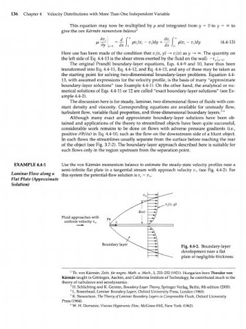
EXAMPLE 4.4-1 Use the von Karman momentum balance to estimate the steady-state velocity profiles near a
semi-infinite flat plate in a tangential stream with approach velocity v x (see Fig. 4.4-2). For
Laminar Flow along a t h i s s y s tem the potential-flow solution is v e = v .
x
Flat Plate (Approximate
Solution)

v x (x, y)

Fluid approaches with
uniform velocity v x

Boundary layer Fig. 4.4-2. Boundary-layer
development near a flat
plate of negligible thickness.

2
Th. von Karman, Zeits. fur angew. Math. u. Mech., 1, 233-252 (1921). Hungarian-born Theodor von
Karman taught in Gottingen, Aachen, and California Institute of Technology; he contributed much to the
theory of turbulence and aerodynamics.
3
H. Schlichting and K. Gersten, Boundary-Layer Theory, Springer Verlag, Berlin, 8th edition (2000).
4
L. Rosenhead, Laminar Boundary Layers, Oxford University Press, London (1963).
5
K. Stewartson, The Theory of Laminar Boundary Layers in Compressible Fluids, Oxford University
Press (1964).
6
W. H. Dorrance, Viscous Hypersonic Flow, McGraw-Hill, New York (1962).