Page 320 - Bird R.B. Transport phenomena

304 Chapter 10 Shell Energy Balances and Temperature Distributions in Solids and Laminar Flow

Sub-
Substance Jstance Substance
01 12 23

t (Ж*

7"
ТУ/У,
a 1 y///.
re,J
2 Fluid 4уу Fluid
2 *^ (
1 ш
ш
H
\^^^ т
^3
Distance,
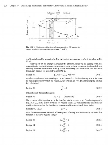
Fig. 10.6-1. Heat conduction through a composite wall, located be-
tween two fluid streams at temperatures T and T .
b
a

coefficients h and h , respectively. The anticipated temperature profile is sketched in Fig.
3
0
10.6-1.
First we set up the energy balance for the problem. Since we are dealing with heat
conduction in a solid, the terms containing velocity in the e vector can be discarded, and
the only relevant contribution is the q vector, describing heat conduction. We first write
the energy balance for a slab of volume WH Ax

Region 01: q \ WH - = 0 (10.6-1)
x x
which states that the heat entering at x must be equal to the heat leaving at x + Ax, since
no heat is produced within the region. After division by WH Ax and taking the limit as
Ax -» 0, we get

Region 01: (10.6-2)
dx
Integration of this equation gives
Region 01: q x = q 0 (a constant) (10.6-3)
The constant of integration, q , is the heat flux at the plane x = x . 0 The development in
0
Eqs. 10.6-1, 2, and 3 can be repeated for regions 12 and 23 with continuity conditions on
q x at interfaces, so that the heat flux is constant and the same for all three slabs:
Regions 01,12, 23: = <7o (10.6-4)

with the same constant for each of the regions. We may now introduce a Fourier's law
for each of the three regions and get

Region 01: (10.6-5)
dx
[
dT
Region 12: (10.6-6)
Region 23: dT (10.6-7)