Page 635 - Bird R.B. Transport phenomena

§20.1 Time Dependent Diffusion 615

This gives on integration

X = Q P exp[-(Z - <p) ]dZ + C 2 (20.1-14)
2
Jo
Combining this result with Eqs. 20.1-11 and 12, we get

2
2
Г exp[-(Z - <p) ]dZ j ' * exp(- W )dW
X(Z) = 1 - - ^ = 1 - — I (20.1-15)
exp[-(Z - <p) ]dZ exp(-W WW
2
2
Jo J -tp
Then we use the definition of the error function and some of the properties of this function, in
particular, -eri(-ip) = erf <p and erf oo = 1 (see §C.6). This leads to the final expression for the
mole fraction distribution: 1
_ e r f ( Z erf l e r f ( Z , )
= t y ) + y =
erf oo + erf (p 1 4- erf <p
To get the function <p(x ), this mole fraction distribution has to be substituted into Eq. 20.1-10.
A0
This gives
2
1 x exp(-<p )
<p = —=- AQ — (20.1-17)
VTT 1 - ^ло 1 + erf <p
Rather than solving this to get <p as a function of x , it is easier to evaluate x A0 as a function of <p:
A0
x A0 = ^ ^ l — — (20.1-18)
2
1 + [VTT(1 + erf <p)<p exp <р Г ]
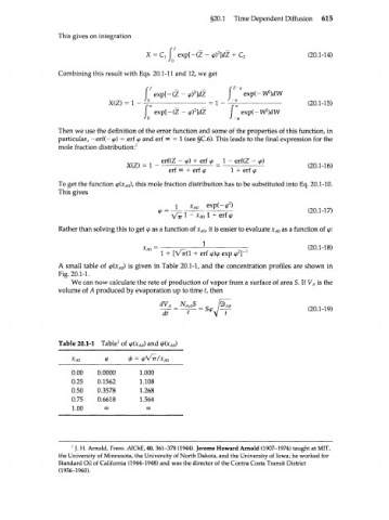
A small table of <p(x ) is given in Table 20.1-1, and the concentration profiles are shown in
A0
Fig. 20.1-1.
We can now calculate the rate of production of vapor from a surface of area S. If V A is the
volume of A produced by evaporation up to time t, then

at

Table 20.1-1 Table 1 of <p(x ) and ф(х )
A0 А0
X A0 ф = <pVjr/x A0

0.00 0.0000 1.000
0.25 0.1562 1.108
0.50 0.3578 1.268
0.75 0.6618 1.564
1.00 00 00

1 J. H. Arnold, Trans. AlChE, 40, 361-378 (1944). Jerome Howard Arnold (1907-1974) taught at MIT,
the University of Minnesota, the University of North Dakota, and the University of Iowa; he worked for
Standard Oil of California (1944-1948) and was the director of the Contra Costa Transit District
(1956-1960).