Page 15 - Using ANSYS for Finite Element Analysis A Tutorial for Engineers

2 • Using ansys for finite element analysis
differential equation or a set of differential equations with a set of cor-
responding boundary and initial conditions whose solution should be
consistent with and accurately represent the physics of the system. These
governing equations represent balance of mass, force, or energy. When
possible, the exact solution of these equations renders detailed behavior of
a system under a given set of conditions.
In situations where the system is relatively simple, it may be possible
to analyze the problem by using some of the classical methods learned
in elementary courses in ordinary and partial differential equations. Far
more frequently, however, there are many practical engineering problems
for which we cannot obtain exact solutions. This inability to obtain an
exact solution may be attributed to either the complex nature of governing
differential equations or the difficulties that arise from dealing with the
boundary and initial conditions. To deal with such problems, we resort to
numerical approximations. In contrast to analytical solutions, which show
the exact behavior of a system at any point within the system, numerical
solutions approximate exact solutions only at discrete points, called nodes.
Due to the complexity of physical systems, some approximation must
be made in the process of turning physical reality into a mathematical
model. It is important to decide at what points in the modeling process
these approximations are made. This, in turn, determines what type of ana-
lytical or computational scheme is required in the solution process. Let us

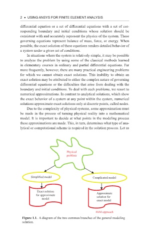
Physical
problem

Simplified model Complicated model

Exact solution Approximate
for approximate solution for
model
exact model

FEM approach
Figure 1.1. A diagram of the two common branches of the general modeling
solution.