Page 18 - Using ANSYS for Finite Element Analysis A Tutorial for Engineers

IntroductIon to FInIte element AnAlysIs • 5
1.1.3 a Brief history of feM

Finite element analysis (FEA) was first developed in 1943 by R. Courant,
who utilized the Ritz method of numerical analysis and minimization
of variational calculus to obtain approximate solutions to vibration
systems. Shortly thereafter, a paper published in 1956 by M. J. Turner,
R. W. Clough, H. C. Martin, and L. J. Topp established a broader definition
of numerical analysis. The paper centered on the “stiffness and deflection
of complex structures.”
By the early 1970s, FEA was limited to expensive mainframe com-
puters generally owned by the aeronautics, automotive, defense, and
nuclear industries. Since the rapid decline in the cost of computers and the
phenomenal increase in computing power, FEA has been developed to an
incredible precision. Present day super computers are now able to produce
accurate results for all kinds of parameters.

1.1.4 the feM analysis Process

A model-based simulation process using FEM consists of a sequence of
steps. This sequence takes two basic configurations depending on the
environment in which FEM is used. These are referred to as the mathe-
matical FEM and the physical FEM.
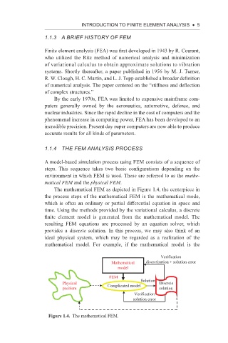
The mathematical FEM as depicted in Figure 1.4, the centerpiece in
the process steps of the mathematical FEM is the mathematical mode,
which is often an ordinary or partial differential equation in space and
time. Using the methods provided by the variational calculus, a discrete
finite element model is generated from the mathematical model. The
resulting FEM equations are processed by an equation solver, which
provides a discrete solution. In this process, we may also think of an
ideal physical system, which may be regarded as a realization of the
mathematical model. For example, if the mathematical model is the

Verification
Mathematical discretization + solution error
model
FEM
Physical Complicated model Solution Discrete
problem solution
Verification
solution error

Figure 1.4. The mathematical FEM.