Page 121 - Well Logging and Formation Evaluation

Integration with Seismic 111

4.500E-07
4.000E-07
3.500E-07
3.000E-07 Shale
Frequency 2.500E-07 Water
Oil
2.000E-07
1.500E-07 Gas
1.000E-07
5.000E-08
0.000E+00
0.00E+00 5.00E+06 1.00E+07 1.50E+07 2.00E+07
Acoustic impedance

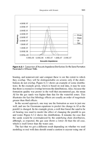
Figure 6.3.1 Comparison of Acoustic Impedance Distributions for the Same Formation
Penetrated in Different Wells

bearing, and nonreservoir) and compare these to see the extent to which
they overlap. They will be distinguishable on seismic only if the distri-
butions do not overlap. Figure 6.3.1 shows an example of some distribu-
tions. In the example given, which is based on real data, it may be seen
that there is extensive overlap between the distributions. Also, because the
formation quality was poorer in the well that encountered gas, the mean
AI for the gas sands was higher than that for the water/oil zones. This
illustrates the fact that lithology effects are usually an order of magnitude
greater than fluid effects.
In the second approach, one may use the formation as seen in just one
well, and use the Gassmann equations to predict the change in AI as the
porefill is changed. In the example given, a well that found the sand to be
oil bearing was used to model the effect of changing the porefill to gas
and water. Figure 6.3.2 shows the distributions. It remains the case that
the sands would be overshadowed by the underlying shale distribution,
although, as expected, the gas case shows a lower AI than the oil case,
which is itself lower than the water case.
The fact that we got a different result depending on whether we used
modeling or real well data should sound a caution to anyone using one of