Page 120 - Well Logging and Formation Evaluation

110 Well Logging and Formation Evaluation

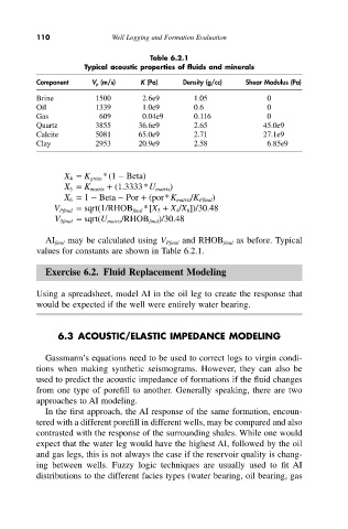
Table 6.2.1
Typical acoustic properties of fluids and minerals
Component V p (m/s) K (Pa) Density (g/cc) Shear Modulus (Pa)
Brine 1500 2.6e9 1.05 0
Oil 1339 1.0e9 0.6 0
Gas 609 0.04e9 0.116 0
Quartz 3855 36.6e9 2.65 45.0e9
Calcite 5081 65.0e9 2.71 27.1e9
Clay 2953 20.9e9 2.58 6.85e9

X 4 = K grain *(1 - Beta)
X 5 = K matrix + (1.3333*U matrix )
X 6 = 1 - Beta - Por + (por*K matrix /K Ffinal )
V Pfinal = sqrt(1/RHOB final *[X 5 + X 4/X 6])/30.48
V Sfinal = sqrt(U matrix /RHOB final )/30.48

AI final may be calculated using V Pfinal and RHOB final as before. Typical
values for constants are shown in Table 6.2.1.

Exercise 6.2. Fluid Replacement Modeling

Using a spreadsheet, model AI in the oil leg to create the response that
would be expected if the well were entirely water bearing.

6.3 ACOUSTIC/ELASTIC IMPEDANCE MODELING

Gassmann’s equations need to be used to correct logs to virgin condi-
tions when making synthetic seismograms. However, they can also be
used to predict the acoustic impedance of formations if the fluid changes
from one type of porefill to another. Generally speaking, there are two
approaches to AI modeling.
In the first approach, the AI response of the same formation, encoun-
tered with a different porefill in different wells, may be compared and also
contrasted with the response of the surrounding shales. While one would
expect that the water leg would have the highest AI, followed by the oil
and gas legs, this is not always the case if the reservoir quality is chang-
ing between wells. Fuzzy logic techniques are usually used to fit AI
distributions to the different facies types (water bearing, oil bearing, gas