Page 118 - Well Logging and Formation Evaluation

108 Well Logging and Formation Evaluation

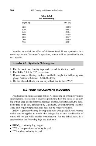
Table 6.1.1
T–Z relationship
Depth (m) TWT (ms)
600 1000.0
620 1009.2
640 1018.4
660 1027.6
680 1036.7
700 1045.9
720 1055.1

In order to model the effect of different fluid fill on synthetics, it is
necessary to use Gassmann’s equations, which will be described in the
next section.

Exercise 6.1. Synthetic Seismogram

1. Use the sonic and density logs to derive AI for the test1 well.
2. Use Table 6.1.1 for T-Z conversion.
3. If you have a filtering package available, apply the following zero
phase Butterworth filter: 10–20–70–90Hz
4. On the filtered AI, do you see any effect due to the OWC?

6.2 FLUID REPLACEMENT MODELING

Fluid replacement is a central part of AI modeling or creating synthetic
seismograms. In essence it involves predicting how the sonic or density
log will change as one porefluid replaces another. Unfortunately, the equa-
tions used to do this, developed by Gassmann, are cumbersome to apply.
They also require input data that may not be readily available.
Below is presented a step-by-step menu for doing a fluid replacement,
which can be applied to model the change due to any combination of
water, oil, or gas with another combination. For the initial case, it is
assumed that the following logs are available:

• RHOB init = density log, in g/cc
• DTP = compressional velocity, in ms/ft
• DTS = shear velocity, in ms/ft