Page 182 - Fluid Power Engineering

Advanced W ind Resource Assessment 155

y Wind
Turbine
k
x 1
d+kx
A 0 A 2
d
ν 0 ν r A r ν 2

Control Volume
x

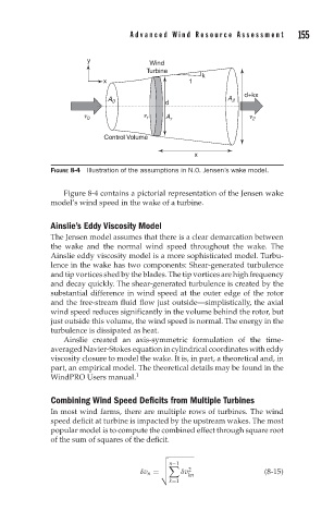
FIGURE 8-4 Illustration of the assumptions in N.O. Jensen’s wake model.

Figure 8-4 contains a pictorial representation of the Jensen wake
model’s wind speed in the wake of a turbine.

Ainslie’s Eddy Viscosity Model
The Jensen model assumes that there is a clear demarcation between
the wake and the normal wind speed throughout the wake. The
Ainslie eddy viscosity model is a more sophisticated model. Turbu-
lence in the wake has two components: Shear-generated turbulence
and tip vortices shed by the blades. The tip vortices are high frequency
and decay quickly. The shear-generated turbulence is created by the
substantial difference in wind speed at the outer edge of the rotor
and the free-stream fluid flow just outside—simplistically, the axial
wind speed reduces significantly in the volume behind the rotor, but
just outside this volume, the wind speed is normal. The energy in the
turbulence is dissipated as heat.
Ainslie created an axis-symmetric formulation of the time-
averaged Navier-Stokes equation in cylindrical coordinates with eddy
viscosity closure to model the wake. It is, in part, a theoretical and, in
part, an empirical model. The theoretical details may be found in the
WindPRO Users manual. 1

Combining Wind Speed Deficits from Multiple Turbines
In most wind farms, there are multiple rows of turbines. The wind
speed deficit at turbine is impacted by the upstream wakes. The most
popular model is to compute the combined effect through square root
of the sum of squares of the deficit.

n−1

δv n = δv 2 (8-15)
kn
k=1