Page 178 - Fluid Power Engineering

Advanced W ind Resource Assessment 151

Return StdDev/ EWS + EWS +
Period Prob ln(-ln EWS Mean 1 × StdDev 2 × StdDev
Year(s) (EWS, n) (prob)) m/s % m/s m/s
1 0.8 −1.50 24.3 4.2 25.3 26.3
5 0.96 −3.20 27.4 6.7 29.2 31.1
10 0.98 −3.90 28.7 7.7 30.9 33.2
25 0.992 −4.82 30.5 8.9 33.2 35.9
50 0.996 −5.52 31.9 9.7 34.9 38.0
100 0.998 −6.21 33.2 10.4 36.7 40.1

Source: Created in WindPRO.
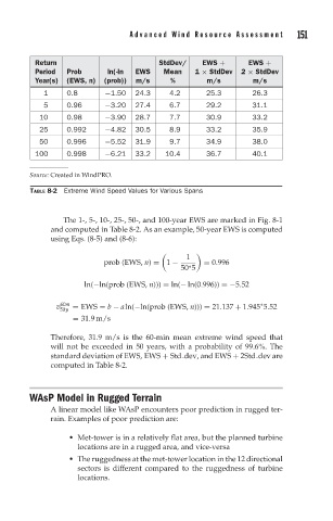
TABLE 8-2 Extreme Wind Speed Values for Various Spans

The 1-, 5-, 10-, 25-, 50-, and 100-year EWS are marked in Fig. 8-1
and computed in Table 8-2. As an example, 50-year EWS is computed
using Eqs. (8-5) and (8-6):

1
prob (EWS, n) = 1 − = 0.996
50 5
∗
ln(−ln(prob (EWS, n))) = ln(− ln(0.996)) =−5.52

∗
v 60m = EWS = b − aln(−ln(prob (EWS, n))) = 21.137 + 1.945 5.52
50y
= 31.9 m/s
Therefore, 31.9 m/s is the 60-min mean extreme wind speed that
will not be exceeded in 50 years, with a probability of 99.6%. The
standard deviation of EWS, EWS + Std dev, and EWS + 2Std dev are
computed in Table 8-2.

WAsP Model in Rugged Terrain
A linear model like WAsP encounters poor prediction in rugged ter-
rain. Examples of poor prediction are:

Met-tower is in a relatively flat area, but the planned turbine

locations are in a rugged area, and vice-versa
The ruggedness at the met-tower location in the 12 directional

sectors is different compared to the ruggedness of turbine
locations.