Page 177 - Fluid Power Engineering

150 Chapter Eight

2 1 1 year(s)
In(-In(P(Extreme Wind Speed))) -1 0 5 year(s) 10 year(s) 25 year(s) 50 year(s)

-2
-3
-4
-5
-6 100 year(s)
20 22 24 26 28 30 32
Extreme Wind Speed
Gumbel Distribution Fitted
Sample Distribution
Estimated Extreme Wind Speeds at Different Return Periods
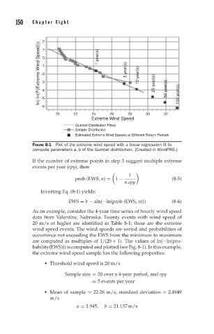
FIGURE 8-1 Plot of the extreme wind speed with a linear regression fit to
compute parameters a, b of the Gumbel distribution. (Created in WindPRO.)
If the number of extreme points in step 3 suggest multiple extreme
events per year (epy), then
1

prob (EWS, n) = 1 − (8-5)
n.epy
Inverting Eq. (8-1) yields:
EWS = b − aln(−ln(prob (EWS, n))) (8-6)
As an example, consider the 4-year time series of hourly wind speed
data from Valentine, Nebraska. Twenty events with wind speed of
20 m/s or higher are identified in Table 8-1; these are the extreme
wind speed events. The wind speeds are sorted and probabilities of
occurrence not exceeding the EWS from the minimum to maximum
are computed as multiples of 1/(20 + 1). The values of ln(−ln(pro-
bability(EWS))) is computed and plotted (see Fig. 8-1). In this example,
the extreme wind speed sample has the following properties:

Threshold wind speed is 20 m/s

Sample size = 20 over a 4-year period, and epy
= 5 events per year

Mean of sample = 22.26 m/s, standard deviation = 2.4949

m/s
a = 1.945, b = 21.137 m/s