Page 176 - Fluid Power Engineering

Advanced W ind Resource Assessment 149

Date EWS Prob (EWS) ln(-ln(Prob))
1/15/1997 20.2 0.05 1.11
1/4/1997 20.3 0.10 0.86
12/30/1998 20.4 0.14 0.67
3/26/1999 20.5 0.19 0.51
7/1/1997 20.6 0.24 0.36
11/22/1998 20.7 0.29 0.23
10/19/1995 20.8 0.33 0.09
12/17/1996 20.8 0.38 −0.04
4/18/1995 20.9 0.43 −0.17
10/11/1997 21.4 0.48 −0.30
4/6/1997 21.7 0.52 −0.44
1/18/1996 22 0.57 −0.58
12/30/1997 22 0.62 −0.73
12/8/1995 22.2 0.67 −0.90
3/24/1996 23.2 0.71 −1.09
10/27/1995 23.5 0.76 −1.30
11/10/1998 24.1 0.81 −1.55
4/25/1996 24.7 0.86 −1.87
10/29/1996 25 0.90 −2.30
2/10/1996 28 0.95 −3.02
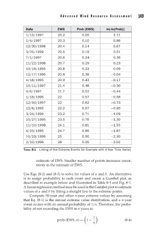
TABLE 8-1 Listing of the Extreme Events for Example with 4-Year Time Series

estimate of EWS. Smaller number of points increases uncer-
tainty in the estimate of EWS.

Use Eqs. (8-2) and (8-3) to solve for values of a and b. An alternative
is to assign probability to each event and create a Gumbel plot, as
described in example below and illustrated in Table 8-1 and Fig. 8-1.
AlinearregressionmethodmaybeusedintheGumbelplottoestimate
values of a and b by fitting a straight line to the extreme points.
Compute 50-year and other n-year extreme values by assuming
that Eq. (8-1) is the annual extreme value distribution, and a n-year
event occurs with an annual probability of 1/n. Therefore, the proba-
bility of not exceeding the EWS in n years is:

1

prob (EWS, n) = 1 − (8-4)
n