Page 206 - Characterization and Properties of Petroleum Fractions - M.R. Riazi

T1: IML
QC: —/—
P1: KVU/KXT
P2: KVU/KXT
AT029-Manual-v7.cls
AT029-04
June 22, 2007
AT029-Manual
186 CHARACTERIZATION AND PROPERTIES OF PETROLEUM FRACTIONS
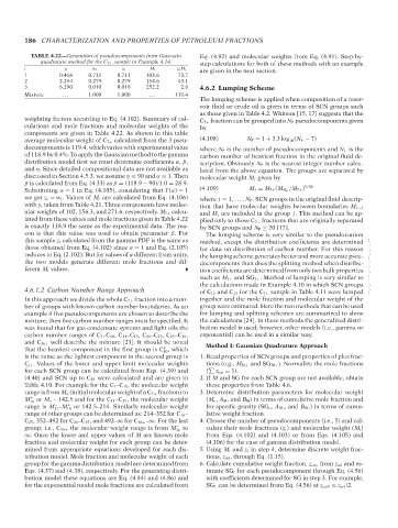
TABLE 4.22—Generation of pseudocomponents from Gaussain
quadrature method for the C 7+ sample in Example 4.14. 21:30 Eq. (4.92) and molecular weights from Eq. (4.91). Step-by-
step calculations for both of these methods with an example
i y i w i z i M i z i M i are given in the next section.
1 0.416 0.711 0.711 103.6 73.7
2 2.294 0.279 0.279 154.6 43.1
3 6.290 0.010 0.010 252.2 2.6 4.6.2 Lumping Scheme
Mixture . . . 1.000 1.000 . . . 119.4
The lumping scheme is applied when composition of a reser-
voir fluid or crude oil is given in terms of SCN groups such
as those given in Table 4.2. Whitson [15, 17] suggests that the
weighting factors according to Eq. (4.102). Summary of cal- C 7+ fraction can be grouped into N P pseudocomponents given
culations and mole fractions and molecular weights of the by
components are given in Table 4.22. As shown in this table
average molecular weight of C 7+ calculated from the 3 pseu- (4.108) N P = 1 + 3.3 log (N + − 7)
10
docomponents is 119.4, which varies with experimental value where N P is the number of pseudocomponents and N + is the
of 118.9 by 0.4%. To apply the Gaussian method to the gamma carbon number of heaviest fraction in the original fluid de-
distribution model first we must determine coefficients α, β, scription. Obviously N P is the nearest integer number calcu-
and η. Since detailed compositional data are not available as lated from the above equation. The groups are separated by
discussed in Section 4.5.3, we assume η = 90 and α = 1. Then molecular weight M j given by
β is calculated from Eq. (4.33) as β = (118.9 − 90)/1.0 = 28.9.
Substituting α = 1 in Eq. (4.105), considering that (α) = 1 (4.109) M j = M 7+ (M N + /M 7+ ) 1/N P
we get z i = w i . Values of M i are calculated from Eq. (4.106) where j = 1,..., N P . SCN groups in the original fluid descrip-
with y i taken from Table 4.21. Three components have molec-
tion that have molecular weights between boundaries M j−1
ular weights of 102, 156.3, and 271.6, respectively. M 7+ calcu- and M j are included in the group j. This method can be ap-
lated from these values and mole fractions given in Table 4.22 plied only to those C 7+ fractions that are originally separated
is exactly 118.9 the same as the experimental data. The rea- by SCN groups and N P ≥ 20 [17].
son is that this value was used to obtain parameter β. For The lumping scheme is very similar to the pseudoization
this sample z i calculated from the gamma PDF is the same as method, except the distribution coefficients are determined
those obtained from Eq. (4.102) since α = 1 and Eq. (2.105) for data on distribution of carbon number. For this reason
reduces to Eq. (2.102). But for values of α different from unity, the lumping scheme generates better and more accurate pseu-
the two models generate different mole fractions and dif- docomponents than does the splitting method when distribu-
ferent M i values. tion coefficients are determined from only two bulk properties --`,```,`,``````,`,````,```,,-`-`,,`,,`,`,,`---
such as M 7+ and SG 7+ . Method of lumping is very similar to
the calculations made in Example 4.10 in which SCN groups
4.6.1.2 Carbon Number Range Approach of C 12 and C 13 for the C 7+ sample in Table 4.11 were lumped
In this approach we divide the whole C 7+ fraction into a num- together and the mole fraction and molecular weight of the
ber of groups with known carbon number boundaries. As an group were estimated. Here the two methods that can be used
example if five pseudocomponents are chosen to describe the for lumping and splitting schemes are summarized to show
mixture, then five carbon number ranges must be specified. It the calculations [24]. In these methods the generalized distri-
was found that for gas condensate systems and light oils the bution model is used; however, other models (i.e., gamma or
carbon number ranges of C 7 –C 10 ,C 11 –C 15 ,C 16 –C 25 ,C 25 –C 36 , exponential) can be used in a similar way.
and C 36+ well describe the mixture [23]. It should be noted Method I: Gaussian Quadrature Approach
that the heaviest component in the first group is C , which
+
10
is the same as the lightest component in the second group is 1. Read properties of SCN groups and properties of plus frac-
−
C . Values of the lower and upper limit molecular weights tions (e.g., M 30+ and SG 30+ ). Normalize the mole fractions
11
for each SCN group can be calculated from Eqs. (4.39) and ( x mi = 1).
(4.40) and SCN up to C 20 were calculated and are given in 2. If M and SG for each SCN group are not available, obtain
Table 4.10. For example for the C 7 –C 10 , the molecular weight these properties from Table 4.6.
range is from M o (initial molecular weight of a C 7+ fraction) to 3. Determine distribution parameters for molecular weight
M 10 or M o – 142.5 and for the C 11 –C 15 , the molecular weight (M o , A M , and B M ) in terms of cumulative mole fraction and
+
range is M –M 15 or 142.5–214. Similarly molecular weight for specific gravity (SG o , A SG , and B SG ) in terms of cumu-
−
+
11
range of other groups can be determined as: 214–352 for C 16 – lative weight fraction.
C 25 , 352–492 for C 26 –C 35 , and 492–∞ for C 36+ –∞. For the last 4. Choose the number of pseudocomponents (i.e., 5) and cal-
group; i.e., C 36+ the molecular weight range is from M 36 to culate their mole fractions (z i ) and molecular weight (M i )
−
∞. Once the lower and upper values of M are known mole from Eqs. (4.102) and (4.103) or from Eqs. (4.105) and
fraction and molecular weight for each group can be deter- (4.106) for the case of gamma distribution model.
mined from appropriate equations developed for each dis- 5. Using M i and z i in step 4, determine discrete weight frac-
tribution model. Mole fraction and molecular weight of each tions, z wi , through Eq. (1.15).
group for the gamma distribution model are determined from 6. Calculate cumulative weight fraction, z cw , from z wi and es-
Eqs. (4.37) and (4.38), respectively. For the generating distri- timate SG i for each pseudocomponent through Eq. (4.56)
bution model these equations are Eq. (4.84) and (4.86) and with coefficients determined for SG in step 3. For example,
for the exponential model mole fractions are calculated from SG 1 can be determined from Eq. (4.56) at z cw1 = z w1 /2.

Copyright ASTM International
Provided by IHS Markit under license with ASTM Licensee=International Dealers Demo/2222333001, User=Anggiansah, Erick
No reproduction or networking permitted without license from IHS Not for Resale, 08/26/2021 21:56:35 MDT