Page 207 - Characterization and Properties of Petroleum Fractions - M.R. Riazi

QC: —/—
T1: IML
P2: KVU/KXT
P1: KVU/KXT
21:30
June 22, 2007
AT029-Manual-v7.cls
AT029-04
AT029-Manual
4. CHARACTERIZATION OF RESERVOIR FLUIDS AND CRUDE OILS 187
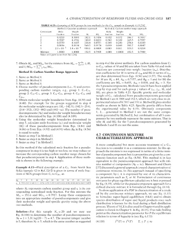
TABLE 4.23—Lumping of SCN groups by two methods for the C 7+ sample in Example 4.15 [24].
Method I: Gaussian quadrature approach Method II: Carbon number range approach
Component Mole Weight Mole Weight
i fraction fraction M i SG i fraction fraction M i SG i
1 0.5218 0.3493 102.1 0.7436 0.532 0.372 106.7 0.7457
2 0.3987 0.4726 180.8 0.8023 0.302 0.328 165.5 0.7957
3 0.0759 0.1645 330.4 0.8591 0.144 0.240 254.4 0.8389
4 0.0036 0.0134 569.5 0.9174 0.019 0.049 392.7 0.8847
5 2.3 × 10 −5 1.4 × 10 −4 950.1 0.9809 0.003 0.011 553.5 0.9214
Mixture 1.0000 1.0000 152.5 0.7905 1.000 1.0000 152.5 0.7908
Taken with permission from Ref. [24].
N P

7. Obtain M av and SG av for the mixture from M av = z j M j in step 4 of the above methods. For carbon numbers from C 7
j=1
N P to C 19 , values of M and SG are taken from Table 4.6 and mole

and 1/SG av = j=1 z wi /SG j .
fractions are converted into weight fraction (x wi ). Distribu-
Method II: Carbon Number Range Approach
tion coefficients for M in terms of x cm and SG in terms of x cw
--`,```,`,``````,`,````,```,,-`-`,,`,,`,`,,`---
1. Same as Method I. are then determined from Eqs. (4.56) and (4.57). The results
2. Same as Method I. for M are M o = 84, A M = 0.7157, and B M = 1 and for SG the
3. Same as Method I. coefficients are SG o = 0.655, A SG = 0.038, and B SG = 3. For
4. Choose number of pseudocomponents (i.e., 5) and corres- the 5 pseudocomponents, Methods I and II have been applied
ponding carbon number ranges, e.g., group 1: C 7 –C 10 , step by step and for each group j values of z mi , z wi , M i , and
group 2: C 11 –C 15 , group 3: C 16 –C 25 , group 4: C 25 –C 36 and SG i are given in Table 4.23. Specific gravity and molecular
C 36+ . weight of C 7+ calculated from pseudocomponents generated
5. Obtain molecular weight boundaries from Eqs. (4.39) and by Method I are 0.7905 and 152.5, which are very close to ex-
(4.40). For example for the groups suggested in step 4 perimental values of 0.7917 and 151.6. Method II gives similar
the molecular weight ranges are: (M o −142.5), (142.5−214), results as shown in Table 4.23. Specific gravity differs from
(214−352), (352−492) and (492−∞). The number of pseu- the experimental value by 0.1%. Obviously components
docomponents (N P ) and molecular weight boundaries may 1, 2, . . . generated in Method I are not the same compo-
also be determined by Eqs. (4.108) and (4.109). nents generated by Method II, but combination of all 5 com-
6. Using the molecular weight boundaries determined in ponents by two methods represent the same mixture. That is
step 5, calculate mole fractions (z i ) and molecular weight why M i and SG i for the 5 pseudocomponents generated by
(M i ) of these pseudocomponents from Eqs. (4.84) and Methods I and II are not the same.
(4.86) or from Eqs. (4.92) and (4.91) when B M in Eq. (4.56)
is equal to unity.
7. Same as step 5 in Method I. 4.7 CONTINUOUS MIXTURE
8. Same as step 6 in Method I. CHARACTERIZATION APPROACH
9. Same as step 7 in Method I.
A more complicated but more accurate treatment of a C 7+
In this method if the calculated mole fraction for a pseudo- fraction is to consider it as a continuous mixture. In this ap-
component in step 6 is too high or too low, we may reduce or proach the mixture is not expressed in terms of a finite num-
increase the corresponding carbon number range chosen for ber of pseudocomponent but its properties are given by a con-
that pseudocomponent in step 4. Application of these meth- tinuous function such as Eq. (4.56). This method is in fact
ods is shown in the following example. equivalent to the pseudocomponent approach but with infi-
nite number of components (N P =∞). Mansoori and Chorn
Example 4.15—Fluid description of a C 7+ from North Sea [27] discussed a general approach toward characterization of
fields (sample 42 in Ref. [24]) is given in terms of mole frac- continuous mixtures. In this approach instead of specifying
tions of SCN groups from C 7 to C 20+ as a component by i, it is expressed by one of its characteris-
tic parameters such as T b or M. Formulation of continuous
N C 7 8 9 10 11 12 13 14 15 16 17 18 19 20+ mixtures for phase equilibrium calculations is best expressed
x i 0.178 0.210 0.160 0.111 0.076 0.032 0.035 0.029 0.022 0.020 0.020 0.016 0.013 0.078 by Eq. (4.15), while for the pseudocomponent approach for a
defined discrete mixture it is formulated through Eq. (4.14).
where N C represents carbon number group and x i is its cor-
responding normalized mole fraction. For this mixture the To show application of a PDF in characterization of a crude
M 7+ = 151.6 and SG 7+ = 0.7917. Lump these components oil by the continuous mixture approach, we use Eq. (4.15)
into an appropriate number of pseudocomponents and give to formulate vapor–liquid equilibrium (VLE) and to obtain
their molecular weight and specific gravity using the above species distribution of vapor and liquid products once such
two methods. distribution is known for the feed during a flash distillation
process. Theory of VLE is discussed in Chapter 6 and its appli-
cation is shown in Chapter 9. In Eq. (4.15), if we take boiling
Solution—For this sample N + = 20 and we may use point as the characterization parameter for P the equilibrium
Eq. (4.108) to determine the number of pseudocomponents. relation in terms of fugacity is (see Eq. 6.173)
N P = 1 + 3.31 log(20 − 7) = 4.7. The nearest integer number
V
L
is 5, therefore N P = 5, which is the same number as suggested (4.110) f (T) = f (T) T ◦ ≤ T ≤∞

Copyright ASTM International
Provided by IHS Markit under license with ASTM Licensee=International Dealers Demo/2222333001, User=Anggiansah, Erick
No reproduction or networking permitted without license from IHS Not for Resale, 08/26/2021 21:56:35 MDT