Page 203 - Characterization and Properties of Petroleum Fractions - M.R. Riazi

QC: —/—
T1: IML
P2: KVU/KXT
P1: KVU/KXT
AT029-Manual-v7.cls
June 22, 2007
21:30
AT029-04
AT029-Manual
4. CHARACTERIZATION OF RESERVOIR FLUIDS AND CRUDE OILS 183
TABLE 4.19—Sample calculations for prediction of distribution of properties of the C 7+
fraction in Example 4.13.
x wi x cw T bi ,K SG i x vi x cv M i x mi I i
No. (1) (2) (3) (4) (5) (6) (7) (8) (9)
1 0.05 0.025 353.8 0.720 0.053 0.026 91.4 0.065 0.244
2 0.05 0.075 359.3 0.730 0.052 0.079 93.9 0.063 0.247
3 0.05 0.125 364.3 0.735 0.052 0.131 96.3 0.062 0.249
i ... ... ... ... ... ... ... ... ...
3. Choose 20 (or more) arbitrary cuts for the mixture with T o = 350 K, A T = 0.1679, and B T = 1.2586. An initial guess
equal weight (or volume) fractions of 0.05 (or less). Then value of SG o = 0.7 is used to calculate A SG and SG distribu-
determine T bi for each cut from Eq. (4.56) and coefficients tion coefficients. Now we divide the whole fraction into 20
from step 2. cuts with equal weight fractions as x wi = 0.05. Similar to cal-
4. Guess an initial value for SG o (lowest value is 0.59). culations shown in Table 4.17, x cw is calculated and then for
5. Calculate 1/J from Eq. (4.80) using SG o and SG 7+ . Then each cut values of T bi and SG i are calculated. From these two
calculate A SG from Eq. (4.79) using Newton’s method or parameters M i and I i are calculated by Eqs. (2.56) and (2.115),
other appropriate procedures. If original TBP is in terms respectively. From x wi and M i mole fractions (x mi ) are calcu-
of x cv , then Eq. (4.76) should be used to determine A SG in lated. Sample calculation for the first few points is given in
Table 4.19 where calculation continues up to i = 20. The co-
terms of x cv.
6. If original TBP is in terms of x cv , find SG distribution from efficients of Eq. (4.56) determined from data in Table 4.19
--`,```,`,``````,`,````,```,,-`-`,,`,,`,`,,`---
Eq. (4.56) in terms of x cv . Then use SG to convert x v to x w are given in Table 4.20. In this method parameter ε 1 = 0.0018
through Eq. (1.16). (step 13), which is less than 0.005 and there is no need to
7. Using values of SG and T b for each cut determine values re-guess SG o . In this set of calculations since initial guess for
of M from Eq. (2.56). SG o is the same as the actual value only one round of cal-
8. Use values of M from step 7 to convert x w into x m through culations was needed. Coefficients given in Table 4.20 have
Eq. (1.15). been used to generate distribution for various properties and
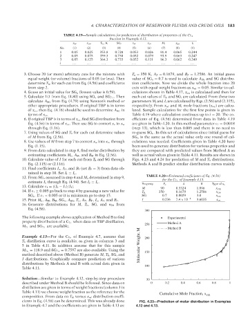
9. From data calculated in step 8, find molar distribution by they are compared with predicted values from Method A as
estimating coefficients M o , A M , and B M in Eq. (2.56). well as actual values given in Table 4.11. Results are shown in
10. Calculate value of I for each cut from T b and SG through Figs. 4.23 and 4.24 for prediction of M and T b distributions.
Eq. (2.115) or (2.116). Methods A and B predict similar distribution curves mainly
11. Find coefficients I o , A I , and B I (set B I = 3) from data ob-
tained in step 10. Set I 1 = I o .
12. From SG o assumed in step 4 and M o determined in step 9, TABLE 4.20—Estimated coefficients of Eq. (4.56)
for the C 7+ of Example 4.13.
estimate I o through Eq. (4.94). Set I 2 = I o . Property A B
13. Calculate ε 1 =|(I 2 − I 1 )/I 1 |. M 90 P o 0.3324 1.096 Type of x c
x cm
14. If ε 1 ≥ 0.005 go back to step 4 by guessing a new value for T b 350 0.1679 1.2586 x cw
SG o .If ε 1 < 0.005 or it is minimum go to step 15. SG 0.7 0.0029 3.0 x cw
15. Print M o , A M , B M ,SG o , A SG , T o , A T , B T , I o , A I , and B I . I 0.236 7.4 × 10 −4 3.6035 x cv
16. Generate distributions for M, T b , SG, and n 20 from
Eq. (4.56).
300
The following example shows application of Method B to find Experimental
property distribution of a C 7+ when data on TBP distillation, Method A
M 7+ and SG 7+ are available. 250 Method B

Example 4.13—For the C 7+ of Example 4.7, assume that 200
T b distillation curve is available, as given in columns 3 and
5 in Table 4.11. In addition assume that for this sample Molecular Weight, M
M 7+ = 118.9 and SG 7+ = 0.7597 are also available. Using the 150
method described above (Method B) generate M, T b , SG, and
I distributions. Graphically compare prediction of various
distributions by Methods A and B with actual data given in
100
Table 4.11.
Solution—Similar to Example 4.12, step-by-step procedure 50
described under Method B should be followed. Since data on 0 0.2 0.4 0.6 0.8 1
distillation are given in terms of weight fractions (column 3 in
Table 4.11) we choose weight fraction as the reference for the Cumulative Mole Fraction, x
composition. From data on T bi versus x wi distribution coeffi- cm
cients in Eq. (4.56) can be determined. This was already done FIG. 4.23—Prediction of molar distribution in Examples
in Example 4.7 and the coefficients are given in Table 4.13 as: 4.12 and 4.13.

Copyright ASTM International
Provided by IHS Markit under license with ASTM Licensee=International Dealers Demo/2222333001, User=Anggiansah, Erick
No reproduction or networking permitted without license from IHS Not for Resale, 08/26/2021 21:56:35 MDT