Page 222 - Characterization and Properties of Petroleum Fractions - M.R. Riazi

P2: IML/FFX
QC: IML/FFX
T1: IML
P1: IML/FFX
AT029-05
August 16, 2007
17:42
AT029-Manual
AT029-Manual-v7.cls
202 CHARACTERIZATION AND PROPERTIES OF PETROLEUM FRACTIONS
pressure is reduced (C to D) or increased (E to F) at constant
T, the first drop of liquid appears at the dew point pressure.
The dewpoint curve is locus of all these dewpoints (dotted).
The dotted lines under the envelope in this figure indicate Γ
constant percent vapor in a mixture of liquid and vapor. The
100% vapor line corresponds to saturated vapor (dewpoint)
curve. The PT diagram for reservoir fluids has a temperature
called cricondentherm temperature (T cric ) as shown in Fig. 5.3. 0
When temperature of a mixture is greater than T cric a gas can- r
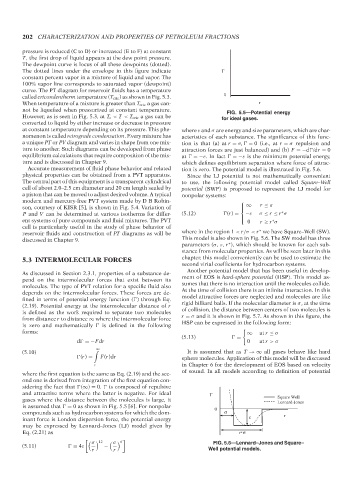
not be liquefied when pressurized at constant temperature. FIG. 5.5—Potential energy
However, as is seen in Fig. 5.3, at T c < T < T cric a gas can be for ideal gases.
converted to liquid by either increase or decrease in pressure
at constant temperature depending on its pressure. This phe- where ε and σ are energy and size parameters, which are char-
nomenon is called retrograde condensation. Every mixture has acteristics of each substance. The significance of this func-
a unique PT or PV diagram and varies in shape from one mix- tion is that (a) at r = σ, = 0 (i.e., at r = σ repulsion and
ture to another. Such diagrams can be developed from phase attraction forces are just balanced) and (b) F =−d /dr = 0
equilibrium calculations that require composition of the mix- at =−ε. In fact =−ε is the minimum potential energy,
ture and is discussed in Chapter 9. which defines equilibrium separation where force of attrac-
Accurate measurement of fluid phase behavior and related tion is zero. The potential model is illustrated in Fig. 5.6.
physical properties can be obtained from a PVT apparatus. Since the LJ potential is not mathematically convenient
The central part of this equipment is a transparent cylindrical to use, the following potential model called Square–Well
cell of about 2.0–2.5 cm diameter and 20 cm length sealed by potential (SWP) is proposed to represent the LJ model for
a piston that can be moved to adjust desired volume. A typical nonpolar systems:
modern and mercury-free PVT system made by D B Robin- ⎧
son, courtesy of KISR [5], is shown in Fig. 5.4. Variation of ⎪ ∞ r ≤ σ
⎨
P and V can be determined at various isotherms for differ- (5.12) (r) = −ε σ ≤ r ≤ r σ
∗
ent systems of pure compounds and fluid mixtures. The PVT ⎪ 0 r ≥ r σ
⎩
∗
cell is particularly useful in the study of phase behavior of
∗
reservoir fluids and construction of PT diagrams as will be where in the region 1 < r/σ < r we have Square–Well (SW).
discussed in Chapter 9. This model is also shown in Fig. 5.6. The SW model has three
parameters (σ, ε, r ), which should be known for each sub-
∗
stance from molecular properties. As will be seen later in this
5.3 INTERMOLECULAR FORCES chapter, this model conveniently can be used to estimate the
second virial coefficients for hydrocarbon systems.
Another potential model that has been useful in develop-
As discussed in Section 2.3.1, properties of a substance de-
pend on the intermolecular forces that exist between its ment of EOS is hard-sphere potential (HSP). This model as-
molecules. The type of PVT relation for a specific fluid also sumes that there is no interaction until the molecules collide.
depends on the intermolecular forces. These forces are de- At the time of collision there is an infinite interaction. In this
fined in terms of potential energy function ( ) through Eq. model attractive forces are neglected and molecules are like
(2.19). Potential energy at the intermolecular distance of r rigid billiard balls. If the molecular diameter is σ, at the time
is defined as the work required to separate two molecules of collision, the distance between centers of two molecules is
from distance r to distance ∞ where the intermolecular force r = σ and it is shown in Fig. 5.7. As shown in this figure, the
is zero and mathematically is defined in the following HSP can be expressed in the following form:
forms: ∞ at r ≤ σ
(5.13) =
d =−Fdr 0 at r >σ
(5.10) ∞ It is assumed that as T →∞ all gases behave like hard
(r) = F(r)dr sphere molecules. Application of this model will be discussed
r in Chapter 6 for the development of EOS based on velocity
of sound. In all models according to definition of potential
where the first equation is the same as Eq. (2.19) and the sec-
ond one is derived from integration of the first equation con-
sidering the fact that (∞) = 0. is composed of repulsive
and attractive terms where the latter is negative. For ideal Γ
gases where the distance between the molecules is large, it Square Well
Lennard-Jones
is assumed that = 0 as shown in Fig. 5.5 [6]. For nonpolar
0
compounds such as hydrocarbon systems for which the dom- σ r
inant force is London dispersion force, the potential energy ε
may be expressed by Lennard–Jones (LJ) model given by
Eq. (2.21) as r*σ

12 6 FIG. 5.6—Lennard–Jones and Square–
σ
σ
(5.11) = 4ε −
r r Well potential models.

--`,```,`,``````,`,````,```,,-`-`,,`,,`,`,,`---
Copyright ASTM International
Provided by IHS Markit under license with ASTM Licensee=International Dealers Demo/2222333001, User=Anggiansah, Erick
No reproduction or networking permitted without license from IHS Not for Resale, 08/26/2021 21:56:35 MDT