
Page 237 - Characterization and Properties of Petroleum Fractions - M.R. Riazi
P. 237
T1: IML
P2: IML/FFX
QC: IML/FFX
P1: IML/FFX
AT029-05
AT029-Manual-v7.cls
August 16, 2007
AT029-Manual
17:42
that for simple fluids it is zero or very small. For example, N 2 ,
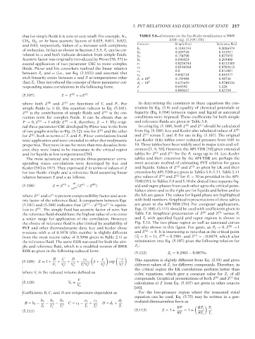
TABLE 5.8—Constants for the Lee-Kesler modification of BWR
EOS—Eq. (5.109) [58].
CH 4 ,O 2 , or Ar have acentric factors of 0.025, 0.011, 0.022, 5. PVT RELATIONS AND EQUATIONS OF STATE 217
and 0.03, respectively. Values of ω increase with complexity Constant Simple fluid Reference fluid
of molecules. In fact as shown in Section 2.5.3, Z c can be cor- b 1 0.1181193 0.2026579
b 2 0.265728 0.331511
related to ω and both indicate deviation from simple fluids.
b 3 0.154790 0.027655
Acentric factor was originally introduced by Pitzer [56, 57] to b 4 0.030323 0.203488
extend application of two-parameter CSC to more complex c 1 0.0236744 0.0313385
fluids. Pitzer and his coworkers realized the linear relation c 2 0.0186984 0.0503618
between Z c and ω (i.e., see Eq. (2.103)) and assumed that c 3 0.0 0.016901
0.041577
0.042724
c 4
such linearity exists between ω and Z at temperatures other d 1 × 10 4 0.155488 0.48736
than T c . They introduced the concept of three-parameter cor- d 2 × 10 4 0.623689 0.0740336
responding states correlations in the following form: β 0.65392 1.226
γ 0.060167 0.03754
(5.107) Z = Z (0) + ωZ (1)
where both Z (0) and Z (1) are functions of T r and P r . For In determining the constants in these equations the con-
simple fluids (ω = 0), this equation reduces to Eq. (5.101). straints by Eq. (5.9) and equality of chemical potentials or
∼
Z (0) is the contribution of simple fluids and Z (1) is the cor- fugacity (Eq. 6.104) between vapor and liquid at saturated
rection term for complex fluids. It can be shown that as conditions were imposed. These coefficients for both simple
P → 0, Z (0) → 1 while Z (1) → 0, therefore, Z → 1. The origi- and reference fluids are given in Table 5.8.
nal three-parameter CSC developed by Pitzer was in the form In using Eq. (5.108), both Z (0) and Z (r) should be calculated
of two graphs similar to Fig. (5.12): one for Z (0) and the other from Eq. (5.109). Lee and Kesler also tabulated values of Z (0)
(1)
for Z , both in terms of T r and P r . Pitzer correlations found and Z (1) versus T r and P r for use in Eq. (5.107). The original
wide application and were extended to other thermodynamic Lee–Kesler (LK) tables cover reduced pressure from 0.01 to
properties. They were in use for more than two decades; how- 10. These tables have been widely used in major texts and ref-
ever, they were found to be inaccurate in the critical region erences [1, 8, 59]. However, the API-TDB [59] gives extended
and for liquids at low temperatures [58]. tables for Z (0) and Z (1) for the P r range up to 14. Lee–Kesler
The most advanced and accurate three-parameter corre- tables and their extension by the API-TDB are perhaps the
sponding states correlations were developed by Lee and most accurate method of estimating PVT relation for gases
Kesler [58] in 1975. They expressed Z in terms of values of Z and liquids. Values of Z (0) and Z (1) as given by LK and their
for two fluids: simple and a reference fluid assuming linear extension by API-TDB are given in Tables 5.9–5.11. Table 5.11
relation between Z and ω as follows: give values of Z (0) and Z (1) for P r > 10 as provided in the API-
TDB [59]. In Tables 5.9 and 5.10 the dotted lines separate liq-
ω
(0)
(5.108) Z = Z (0) + (Z (r) − Z ) uid and vapor phases from each other up to the critical point.
ω (r)
Values above and to the right are for liquids and below and to
where Z (r) and ω (r) represent compressibility factor and acen- the left are gases. The values for liquid phase are highlighted
tric factor of the reference fluid. A comparison between Eqs. with bold numbers. Graphical representations of these tables
(0)
(5.107) and (5.108) indicates that [Z (r) − Z ]/ω (r) is equiva- are given in the API-TDB [59]. For computer applications,
(1)
lent to Z . The simple fluid has acentric factor of zero, but Eqs. (5.108)–(5.111) should be used with coefficients given in
the reference fluid should have the highest value of ω to cover Table 5.8. Graphical presentation of Z (0) and Z (1) versus P r
a wider range for application of the correlation. However, and T r with specified liquid and vapor regions is shown in
the choice of reference fluid is also limited by availability of Fig. 5.13. The two-phase region as well as saturated curves
PVT and other thermodynamic data. Lee and Kesler chose are also shown in this figure. For gases, as P r → 0, Z (0) →1
n-octane with ω of 0.3978 (this number is slightly different and Z (1) → 0. It is interesting to note that at the critical point
from the most recent value of 0.3996 given in Table 2.1) as (T r = P r = 1), Z (0) = 0.2901, and Z (1) =−0.0879, which after
the reference fluid. The same EOS was used for both the sim- substitution into Eq. (5.107) gives the following relation for
ple and reference fluid, which is a modified version of BWR Z c :
EOS as given in the following reduced form:
(5.112) Z c = 0.2901 − 0.0879ω
B C D c 4 γ −γ This equation is slightly different from Eq. (2.93) and gives
(5.109) Z = 1 + + 2 + 5 + 3 2 β + 2 exp 2
V r V r V r T V r V r V r different values of Z c for different compounds. Therefore, in
r
the critical region the LK correlations perform better than
where V r is the reduced volume defined as cubic equations, which give a constant value for Z c of all
V compounds. Graphical presentations of both Z (0) and Z (1) for
(5.110) V r = calculation of Z from Eq. (5.107) are given in other sources
V c
[60].
Coefficients B, C, and D are temperature-dependent as For the low-pressure region where the truncated virial
equation can be used, Eq. (5.75) may be written in a gen-
--`,```,`,``````,`,````,```,,-`-`,,`,,`,`,,`---
b 2 b 3 b 4 c 2 c 3 d 2 eralized dimensionless form as
B = b 1 − − 2 − 3 C = c 1 − + 3 D = d 1 +
T r T T T r T T r
r r r BP BP c P r
(5.111) (5.113) Z = 1 + RT = 1 + RT c T r
Copyright ASTM International
Provided by IHS Markit under license with ASTM Licensee=International Dealers Demo/2222333001, User=Anggiansah, Erick
No reproduction or networking permitted without license from IHS Not for Resale, 08/26/2021 21:56:35 MDT