Page 362 - Characterization and Properties of Petroleum Fractions - M.R. Riazi

P1: JDW
14:25
AT029-Manual-v7.cls
AT029-Manual
AT029-08
June 22, 2007
342 CHARACTERIZATION AND PROPERTIES OF PETROLEUM FRACTIONS
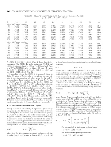
TABLE 8.5—Values of k r (1) and k r (2) for Eq. (8.39). (Taken with permission from Ref. [32].)
k 1 2
k r = = (0.5 − ω)k + ωk r (8.39)
r
k c
P r
T r 0.2 0.5 1.0 1.5 2.0 3.0 4.0 6.0 8.0 10.0
(1)
Values of k r versus T r and P r
1.00 1.1880 1.3307 2.0000 4.1517 4.4282 4.7900 5.2140 5.7989 6.2080 6.5132
1.05 1.3002 1.3640 1.8922 3.2806 3.7990 4.4915 4.7590 5.2817 5.7710 6.2040
1.10 1.4300 1.4810 1.8660 2.5989 3.3334 4.1068 4.4746 4.9502 5.3740 5.8812
1.15 1.5182 1.5365 1.8356 2.2978 2.9769 3.8583 4.4676 4.9404 5.3734 5.8760
1.20 1.8311 1.8956 2.1200 2.3983 2.8809 3.5626 4.2067 4.9285 5.3731 5.8699
1.40 2.1838 2.2520 2.3589 2.5291 2.7120 3.3000 4.0020 4.6327 5.2404 5.7656
1.60 2.5971 2.6589 2.7305 2.8572 3.0035 3.3760 3.8239 4.4385 4.8967 5.3031
2.00 3.6763 3.6984 3.7418 3.9161 3.9594 4.1370 4.3768 4.7138 5.0462 5.3614
3.00 6.9896 7.0010 7.0310 7.0617 7.1079 7.1452 7.2197 7.4077 7.5915 7.7685
(2)
Values of k r versus T r and P r
1.00 1.6900 1.6990 2.0000 2.0619 2.3112 2.3140 2.3160 2.3180 2.3210 2.3212
1.05 1.7200 1.7290 1.8100 1.8170 2.1318 2.1912 2.3010 2.8380 2.3398 2.3400
1.10 1.8001 1.8211 1.8300 1.8310 1.9672 2.1384 2.1369 2.3614 2.3988 2.4105
1.15 2.0599 2.0601 2.0661 2.0700 2.0801 2.1269 2.2246 2.3780 2.4618 2.4622
1.20 2.1441 2.1539 2.1629 2.1681 2.1689 2.1901 2.2319 2.3981 2.4640 2.4701
1.40 2.6496 2.6772 2.6865 2.6889 2.6900 2.6911 2.7001 2.7119 2.8079 2.8810
1.60 3.2184 3.2448 3.2559 3.2886 3.3142 8.8292 3.3343 3.3352 3.8869 3.4525
2.00 4.5222 4.5330 4.5465 4.6871 4.6378 4.7108 4.8148 4.8119 4.8850 4.9885
3.00 8.4002 8.4158 8.4234 8.4503 8.4504 8.5038 8.6083 8.6204 8.6732 8.7454
T = 573.2 K (300 C) k = 0.048 W/m · K. From Lee–Kesler hydrocarbons, thermal conductivity varies linearly with tem-
◦
◦
correlation (Eq. 5.107), the molar volume at 573.2 K and perature:
3
100 bar is calculated as Z = 0.59 or V = 281 cm /mol. Thus
ρ r = V c /V = 313.05/281 = 1.114. Since 0.5 <ρ r < 2, from (8.41) k = A + BT
Eq. (8.38)
= 151.82, A = 2.702, B = 0.67, C =−1.069, and Coefficients A and B can be determined if at least two data
k = 0.048 + 0.017 = 0.065 W/m · K. points on thermal conductivity are available. Values of ther-
To calculate k from Eq. (8.39), k c is required. Since in mal conductivity of some compounds at melting and boiling
Table 8.4 value of k c for n-C 5 is not given, one can ob- points are given in Table 8.6, as given in the API-TDB [5]. Liq-
tain it from interpolation of values given for C 4 and C 7 uid thermal conductivity of several n-paraffins as calculated
by assuming a linear relation between k c and T c . For C 4 , from Eq. (8.41) (or Eq. 8.42) is shown in Fig. 8.4.
k c = 0.0478 and T c = 425.2 K and for C 7 , k c = 0.0535 and If values of thermal conductivity at melting and boiling
T c = 540.2 K. For C 5 with T c = 469.7 by linear interpolation, points are taken as reference points, then Eq. (8.41) can be
k c = [(0.0535 − 0.0478)/(540.2 − 425.2)] × (469.7 − 425.2) + used to obtain value of thermal conductivity at any other tem-
0.0478 = 0.05 W/m · K. Extrapolation between values of k c for perature:
C 3 and C 4 to k c of C 5 gives a slightly different value. At T and P
of interest, T r = 1.22 and P r = 2.97. From Table 8.5, k (1) = 3.5 (8.42) k = k + k − k L T − T M
L
L
L
r

and k (2) = 2.2. From Eq. (8.39), k r = 1.42 and k = 0.05 × T M b M
r T b − T M
1.42 = 0.071 W/m · K. Stiel–Thodos method varies by 8.5%
from Riazi–Faghri method, which represents a reasonable where T M and T b are normal melting (or triple) and boiling
L
L
deviation. In this case the Stiel–Thodos method is more ac- points, respectively. k M and k are values of liquid thermal
b
L
curate since the value of k is calculated more accurately. conductivity at T M and T b , respectively. k is value of liquid
T
◦
thermal conductivity at temperature T. According to API-TDB
8.2.2 Thermal Conductivity of Liquids [5] this equation can predict values of liquid thermal conduc-
tivity of pure compounds up to pressure of 35 bar with an
Theory of thermal conductivity of liquids was proposed by accuracy of about 5% [5]. There are a number of generalized
Bridgman [1]. In this theory, it is assumed that molecules correlations developed for prediction of thermal conductivity
are arranged as cubic lattice with center-to-center spacing of pure hydrocarbon liquids. The Riedel method is included
of (V/N A ) 1/3 , in which V is the molar volume and N A is the in the API-TDB [5]:
Avogadro number. Furthermore, it is assumed that energy ⎡ ⎤
is transferred from one lattice to another at the speed of n 3 + 20 (1 − T r) 2/3
L
sound, c s . This theory provides the basis of prediction of ther- (8.43) k = CM ⎢
2/3 ⎥
L
⎦
⎣
mal conductivity of liquids. For monoatomic liquids the fol- V 25 3 + 20 1 − 298.15
T r
lowing relation can be obtained from this theory [1]:
2 For unbranched, straight-chain hydrocarbons,
3
N A
(8.40) k = 3 k B c s n = 1.001 and C = 0.1811
V
where k B is the Boltzman’s constant and methods of calcula- For branched and cyclic hydrocarbons,
tion of c s have been discussed in Section 6.9. For pure liquid n = 0.7717 and C = 0.4407
--`,```,`,``````,`,````,```,,-`-`,,`,,`,`,,`---
Copyright ASTM International
Provided by IHS Markit under license with ASTM Licensee=International Dealers Demo/2222333001, User=Anggiansah, Erick
No reproduction or networking permitted without license from IHS Not for Resale, 08/26/2021 21:56:35 MDT