Page 236 - Mechanical Behavior of Materials

Section 6.2 Plane Stress 237

y ' y
θ
τ θ x '
σ σ
x 1
cos θ θ + 90 o
x
sin θ
τ
xy
σ
y
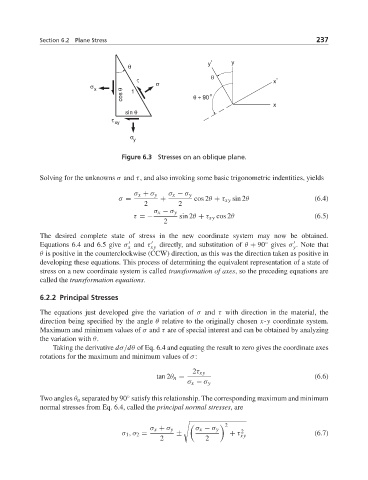
Figure 6.3 Stresses on an oblique plane.

Solving for the unknowns σ and τ, and also invoking some basic trigonometric indentities, yields

σ x + σ y σ x − σ y
σ = + cos 2θ + τ xy sin 2θ (6.4)
2 2
σ x − σ y
τ =− sin 2θ + τ xy cos 2θ (6.5)
2
The desired complete state of stress in the new coordinate system may now be obtained.

◦
Equations 6.4 and 6.5 give σ and τ directly, and substitution of θ + 90 gives σ . Note that
x xy y
θ is positive in the counterclockwise (CCW) direction, as this was the direction taken as positive in
developing these equations. This process of determining the equivalent representation of a state of
stress on a new coordinate system is called transformation of axes, so the preceding equations are
called the transformation equations.
6.2.2 Principal Stresses

The equations just developed give the variation of σ and τ with direction in the material, the
direction being specified by the angle θ relative to the originally chosen x-y coordinate system.
Maximum and minimum values of σ and τ are of special interest and can be obtained by analyzing
the variation with θ.
Taking the derivative dσ/dθ of Eq. 6.4 and equating the result to zero gives the coordinate axes
rotations for the maximum and minimum values of σ:

2τ xy
tan 2θ n = (6.6)
σ x − σ y

Two angles θ n separated by 90 satisfy this relationship. The corresponding maximum and minimum
◦
normal stresses from Eq. 6.4, called the principal normal stresses,are

2

σ x + σ y σ x − σ y
2
σ 1 ,σ 2 = ± + τ xy (6.7)
2 2