Page 136 - Introduction to Statistical Pattern Recognition

118 Introduction to Statistical Pattern Recognition

E{sl*) =aEz + b(1 -E;?). (3.201)
On the other hand, since (3.198) is a random sum, it is known that

E(slo;} =E{E(slm,oi}} =E{mqiIoj} =E(mIoj}qj , (3.202)
I
where E { h (Xi) mi ] is equal to qj, regardless of j. Thus, the average number
of observations needed to reach the decisions is
~(l -E*) +bel
E(mlm,) = , (3.203)
rll
+
UE~ b(l - 2 )
~
E(mly) = (3.204)
rl2
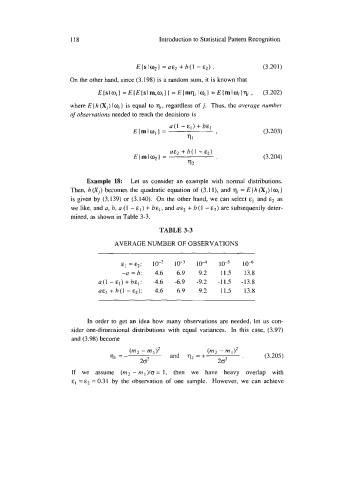
Example 18: Let us consider an example with normal distributions.
Then, h (Xi) becomes the quadratic equation of (3.1 l), and qj = E 1 h (Xi) Io; }
is given by (3.139) or (3.140). On the other hand, we can select and &2 as
we like, and a, b, a (1 - E I ) + b~,, and + b (1 - E*) are subsequently deter-
mined, as shown in Table 3-3.

TABLE 3-3

AVERAGE NUMBER OF OBSERVATIONS

el =e2: io-* io4 10-~ io4
-a = b 4.6 6.9 9.2 11.5 13.8
a(l-~I)+h~l: -4.6 -6.9 -9.2 -11.5 -13.8
+
UE~ h(1 - ~2): 4.6 6.9 9.2 11.5 13.8

In order to get an idea how many observations are needed, let us con-
sider one-dimensional distributions with equal variances. In this case, (3.97)
and (3.98) become
(1112 - md2 (m2 - m I)*
ql=- and q2 =+ (3.205)
202 202
If we assume (m2 - ml)/a= 1, then we have heavy overlap with
=
E] =E~ 0.31 by the observation of one sample. However, we can achieve