Page 352 - Introduction to Statistical Pattern Recognition

334 Introduction to Statistical Pattern Recognition

mates [(XY)), and then incrementing the value of t through this list,
keeping track of the number of errors for each value oft.
(d) Classify the sample Xf’ using the original density estimates of
(7.57) and the value of r found in Step (c):

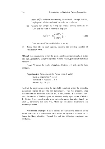
(7.61)

Count an error if the decided class is not 0,.
(3) Repeat Step (2) for each sample, counting the resulting number of
classification errors.

Although this procedure is by far the most complex computationally, it is the
only true L procedure, and gives the most reliable results, particularly for small
values of r.
Figure 7-9 shows the results of applying Options 1, 3, and 4 to the three
test cases.

Experiment 6: Estimation of the Parzen error, L and R
Same as Experiment 4 except
Threshold: r - Options 1, 3, 4
Results: Fig. 7-9 [ 121

In all of the experiments, using the threshold calculated under the normality
assumption (Option 1) gave the best performance. This was expected, since
both the data and the kernel function are, in fact, normal. It is notable, how-
ever, that the use of Option 4 gave performance nearly equal to that of Option
1. Option 3 gave good results also, but performance degraded sharply for
small I’, particularly for Data 1-41, where the covariance determinants are
extremely different.

Non-normal example: It is of interest to examine the behavior of the
Parzen classifier in a non-normal case where the quadratic classifier is no
longer the Bayes classifier. Toward this end, the following experiment was
conducted.