Page 354 - Introduction to Statistical Pattern Recognition

336 Introduction to Statistical Pattern Recognition

densities becomes a quadratic classifier, resulting in the error much higher than
the Bayes error. As the result, the curves of Fig. 7-10 is significantly different
from the ones of Fig. 7-9, indicating that the selection of a proper r for non-
normal cases could be more critical than the one for normal cases. Neverthe-
less, the Parzen classification does provide usable bounds on the Bayes error.

Selection of the kernel shape: An alternative way of compensating for
the biases of the error estimate is the selection of the kernel shape. Equations
(7.50) and (7.51) suggest that, if the kernel covariances are selected such that
a, (X) = a2(X), all terms which are independent of the sample size may be
eliminated from the bias expression. Hence, we must find positive definite
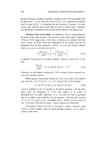
matrices A I and A2 such that, from (6.13),

(7.62)

In general, V2pi(X)/pi(X)'s are hard to obtain. However, when pi(X) is nor-
mal,

(7.63)

Therefore, we may obtain a solution of (7.62) in terms of these expected vec-
tors and covariance matrices.

Before going to the general solution of (7.62), let us look at the simplest
case, where Z, = C2 = C and A = A2 = C. Using (7.63), (7.62) becomes

(X-M I )Y (X-M ' ) = (X-M2)Y (X-M2) (7.64)
which is satisfied by the X's located on the Bayes boundary. On the other
hand, since the integration of (7.45) with respect to w results in
1
J[E(AhJbh)+(1/2)E(Ah2 d6(h)/dhl (P,p,-f *p2)dX, the bias is generated
only by E { Ah(X) I and E{ Ah2(X) 1 on the boundary. Therefore, the selection
of A = A2 = C seems to be a reasonable choice. Indeed, the error curve of
Fig. 7-7(a) shows little bias for large r, without adjusting the threshold.
The general solution of (7.62) is very hard to obtain. However, since
(7.62) is a scaler equation, there are many possible solutions. Let us select a
solution of the form